DENSITY MATRICES traces Operators and Measurements Lectures 10

DENSITY MATRICES, traces, Operators and Measurements Lectures 10 , 11 and 12 Richard Cleve Sources: Michael A. Nielsen Michele Mosca 1

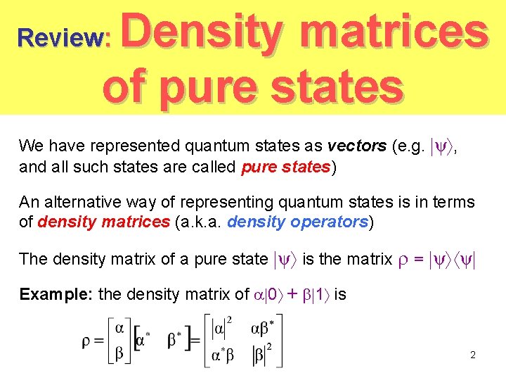
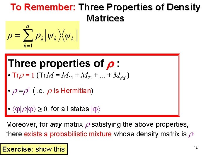
Density matrices of pure states Review: We have represented quantum states as vectors (e. g. ψ , and all such states are called pure states) An alternative way of representing quantum states is in terms of density matrices (a. k. a. density operators) The density matrix of a pure state ψ is the matrix = ψ ψ Example: the density matrix of 0 + 1 is 2

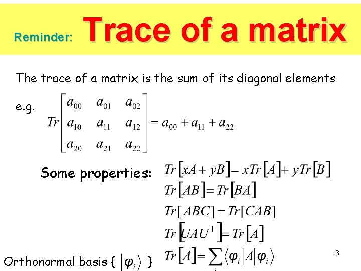
Reminder: Trace of a matrix The trace of a matrix is the sum of its diagonal elements e. g. Some properties: Orthonormal basis { } 3

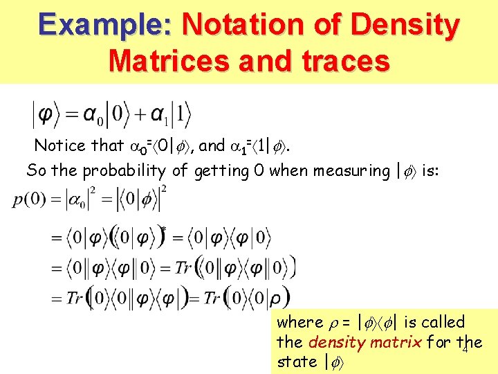
Example: Notation of Density Matrices and traces Notice that 0= 0| , and 1= 1| . So the probability of getting 0 when measuring | is: where = | | is called the density matrix for the 4 state |

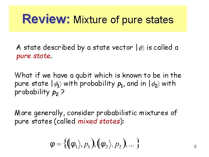
Review: Mixture of pure states A state described by a state vector | is called a pure state. What if we have a qubit which is known to be in the pure state | 1 with probability p 1, and in | 2 with probability p 2 ? More generally, consider probabilistic mixtures of pure states (called mixed states): 5

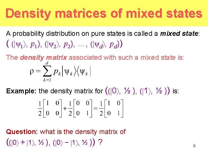
Density matrices of mixed states A probability distribution on pure states is called a mixed state: ( ( ψ1 , p 1), ( ψ2 , p 2), …, ( ψd , pd)) The density matrix associated with such a mixed state is: Example: the density matrix for (( 0 , ½ ), ( 1 , ½ )) is: Question: what is the density matrix of (( 0 + 1 , ½ ), ( 0 − 1 , ½ )) ? 6

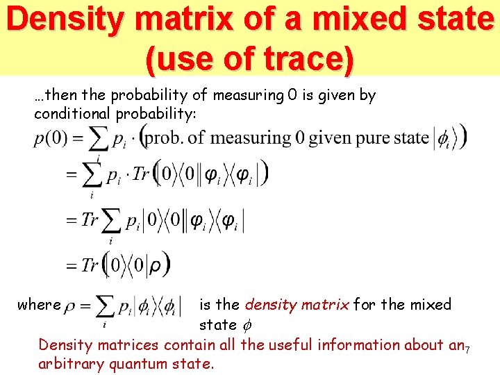
Density matrix of a mixed state (use of trace) …then the probability of measuring 0 is given by conditional probability: where is the density matrix for the mixed state Density matrices contain all the useful information about an 7 arbitrary quantum state.

Recap: operationally indistinguishable states Since these are expressible in terms of density matrices alone (independent of any specific probabilistic mixtures), states with identical density matrices are operationally indistinguishable 8

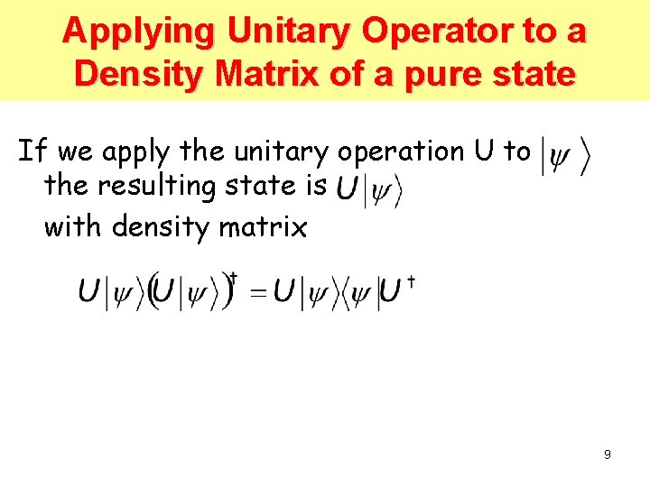
Applying Unitary Operator to a Density Matrix of a pure state If we apply the unitary operation U to the resulting state is with density matrix 9

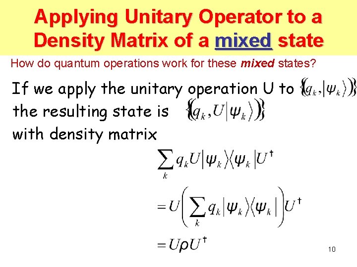
Applying Unitary Operator to a Density Matrix of. Matrix a mixed state How do quantum operations work for these mixed states? If we apply the unitary operation U to the resulting state is with density matrix 10

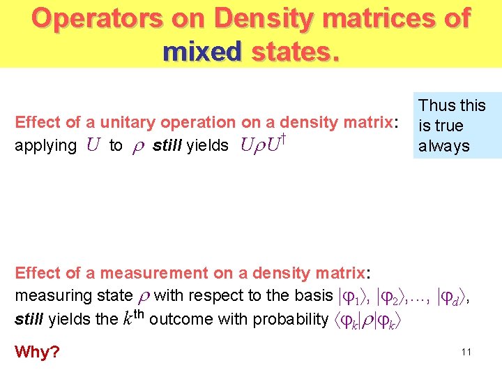
Operators on Density matrices of mixed states. Effect of a unitary operation on a density matrix: † applying U to still yields U U Thus this is true always Effect of a measurement on a density matrix: measuring state with respect to the basis 1 , 2 , . . . , d , still yields the k th outcome with probability k k Why? 11

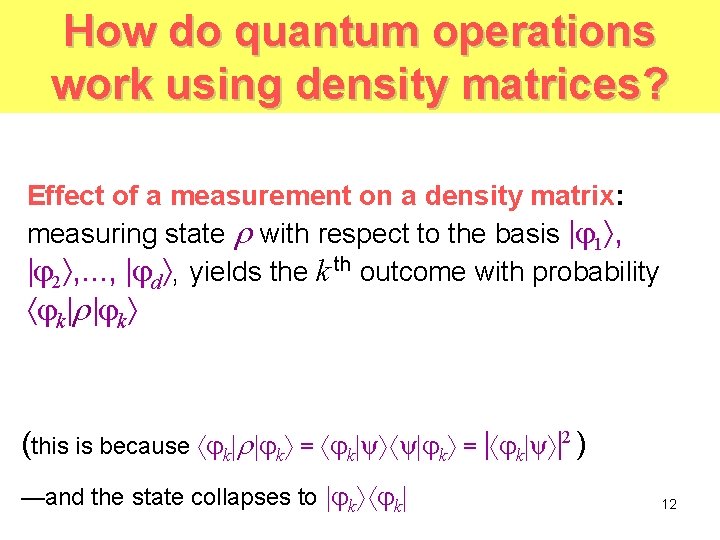
How do quantum operations work using density matrices? Effect of a measurement on a density matrix: measuring state with respect to the basis 1 , 2 , . . . , d , yields the k th outcome with probability k k (this is because k k = k ψ ψ k = k ψ 2 ) —and the state collapses to k k 12

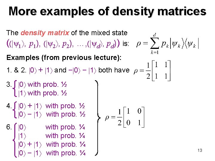
More examples of density matrices The density matrix of the mixed state (( ψ1 , p 1), ( ψ2 , p 2), …, ( ψd , pd)) is: Examples (from previous lecture): 1. & 2. 0 + 1 and − 0 − 1 both have 3. 0 with prob. ½ 1 with prob. ½ 4. 0 + 1 with prob. ½ 0 − 1 with prob. ½ 6. 0 1 0 + 1 0 − 1 with prob. ¼ 13

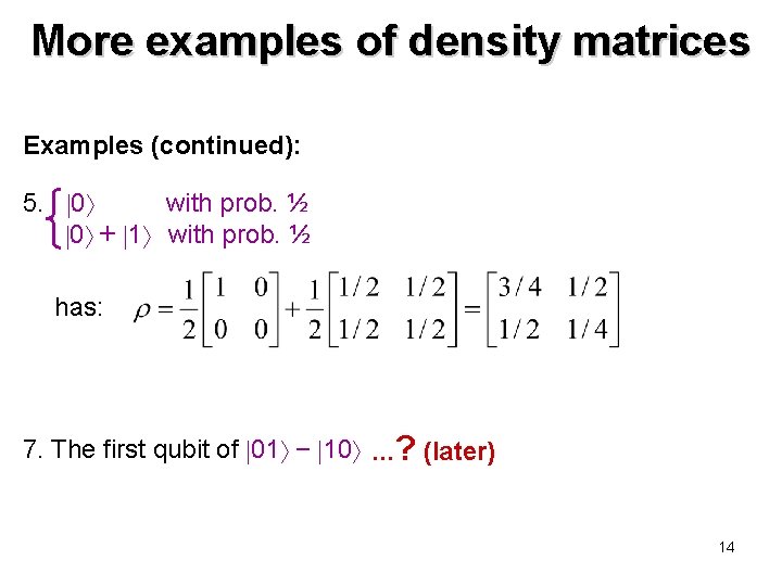
More examples of density matrices Examples (continued): 5. 0 with prob. ½ 0 + 1 with prob. ½ has: 7. The first qubit of 01 − 10 . . . ? (later) 14

To Remember: Three Properties of Density Matrices Three properties of : • Tr = 1 (Tr M = M 11 + M 22 +. . . + Mdd ) • = † (i. e. is Hermitian) • 0, for all states Moreover, for any matrix satisfying the above properties, there exists a probabilistic mixture whose density matrix is Exercise: show this 15

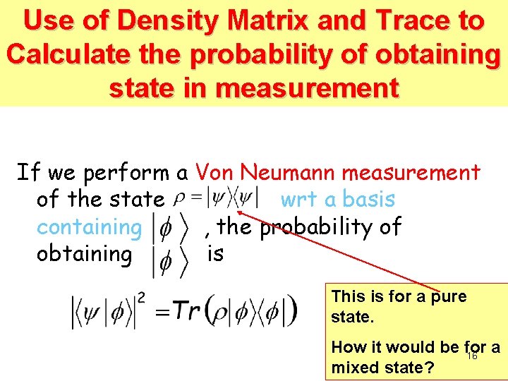
Use of Density Matrix and Trace to Calculate the probability of obtaining state in measurement If we perform a Von Neumann measurement of the state wrt a basis containing , the probability of obtaining is This is for a pure state. How it would be for a 16 mixed state?

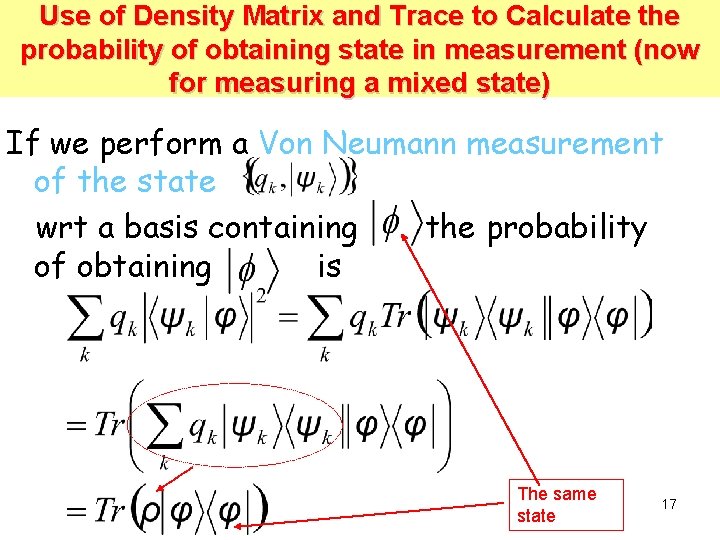
Use of Density Matrix and Trace to Calculate the probability of obtaining state in measurement (now Densitya. Matrix for measuring mixed state) If we perform a Von Neumann measurement of the state wrt a basis containing the probability of obtaining is The same state 17

Conclusion: Density Matrix Has Complete Information In other words, the density matrix contains all the information necessary to compute the probability of any outcome in any future measurement. 18

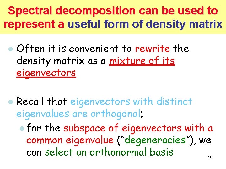
Spectral decomposition can be used to represent a useful form of density matrix l l Often it is convenient to rewrite the density matrix as a mixture of its eigenvectors Recall that eigenvectors with distinct eigenvalues are orthogonal; l for the subspace of eigenvectors with a common eigenvalue (“degeneracies”), we can select an orthonormal basis 19

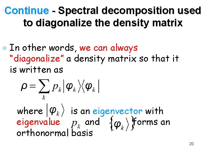
Continue - Spectral decomposition used to diagonalize the density matrix l In other words, we can always “diagonalize” a density matrix so that it is written as where is an eigenvector with eigenvalue and forms an orthonormal basis 20

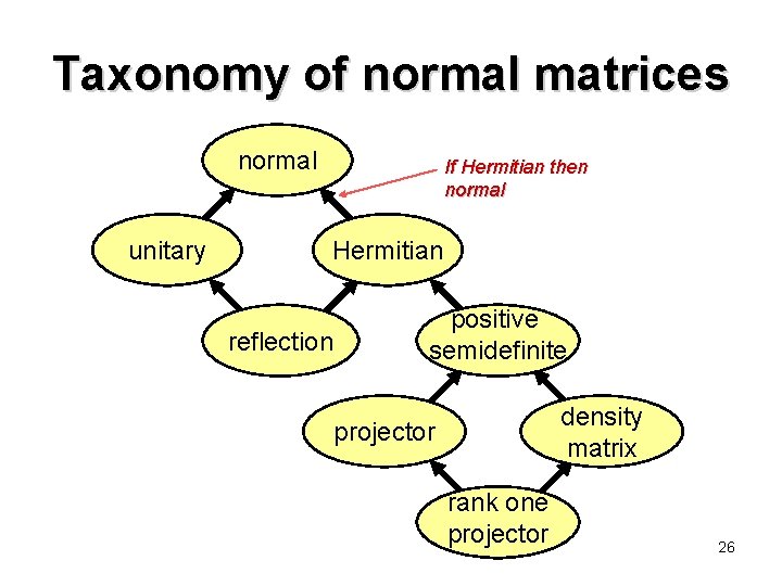
Taxonomy of various normal matrices 21

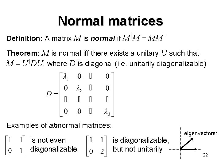
Normal matrices Definition: A matrix M is normal if M†M = MM† Theorem: M is normal iff there exists a unitary U such that M = U†DU, where D is diagonal (i. e. unitarily diagonalizable) Examples of abnormal matrices: is not even diagonalizable is diagonalizable, but not unitarily eigenvectors: 22

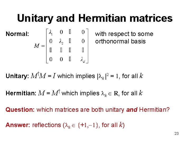
Unitary and Hermitian matrices Normal: with respect to some orthonormal basis Unitary: M†M = I which implies | k |2 = 1, for all k Hermitian: M = M† which implies k R, for all k Question: which matrices are both unitary and Hermitian? Answer: reflections ( k {+1, 1}, for all k) 23

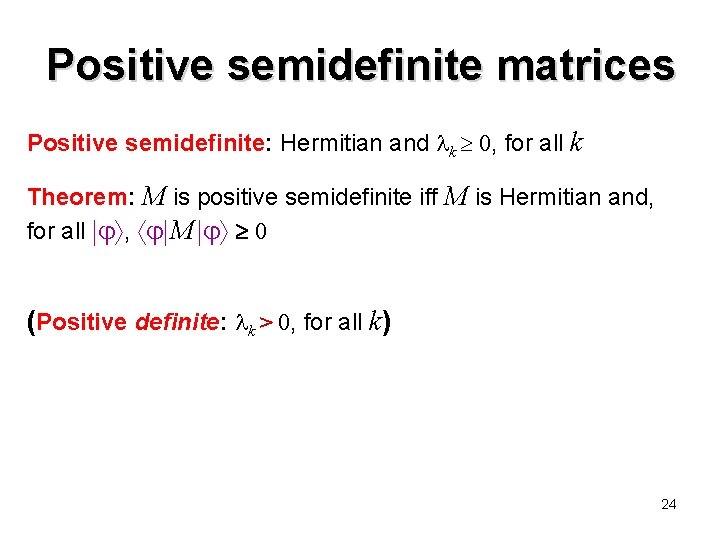
Positive semidefinite matrices Positive semidefinite: Hermitian and k 0, for all k Theorem: M is positive semidefinite iff M is Hermitian and, for all , M 0 (Positive definite: k > 0, for all k) 24

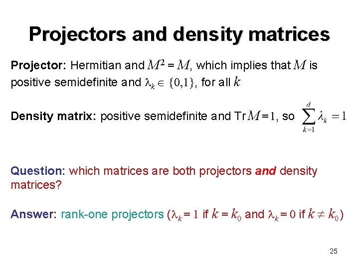
Projectors and density matrices Projector: Hermitian and M 2 = M, which implies that M is positive semidefinite and k {0, 1}, for all k Density matrix: positive semidefinite and Tr M = 1, so Question: which matrices are both projectors and density matrices? Answer: rank-one projectors ( k = 1 if k = k 0 and k = 0 if k k 0 ) 25

Taxonomy of normal matrices normal unitary If Hermitian then normal Hermitian reflection positive semidefinite density matrix projector rank one projector 26

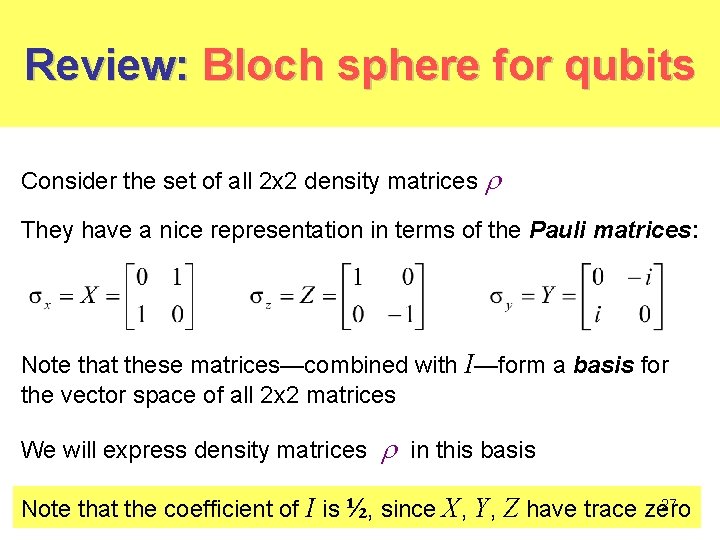
Review: Bloch sphere for qubits Consider the set of all 2 x 2 density matrices They have a nice representation in terms of the Pauli matrices: Note that these matrices—combined with I—form a basis for the vector space of all 2 x 2 matrices We will express density matrices in this basis 27 Note that the coefficient of I is ½, since X, Y, Z have trace zero

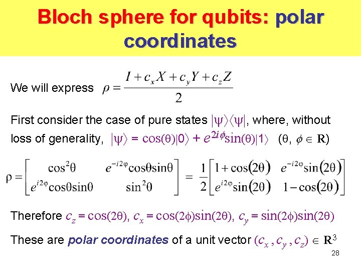
Bloch sphere for qubits: polar coordinates We will express First consider the case of pure states , where, without loss of generality, = cos( ) 0 + e 2 i sin( ) 1 ( , R) Therefore cz = cos(2 ), cx = cos(2 )sin(2 ), cy = sin(2 ) These are polar coordinates of a unit vector (cx , cy , cz) R 3 28

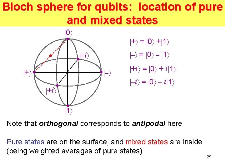
Bloch sphere for qubits: location of pure and mixed states 0 + = 0 + 1 – = 0 – 1 –i + – +i = 0 + i 1 –i = 0 – i 1 1 Note that orthogonal corresponds to antipodal here Pure states are on the surface, and mixed states are inside (being weighted averages of pure states) 29

General quantum operations Decoherence, partial traces, measurements. 30

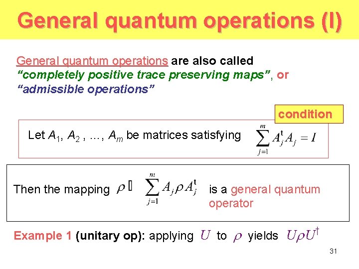
General quantum operations (I) General quantum operations are also called “completely positive trace preserving maps”, or “admissible operations” condition Let A 1, A 2 , …, Am be matrices satisfying Then the mapping is a general quantum operator Example 1 (unitary op): applying U to yields U U† 31

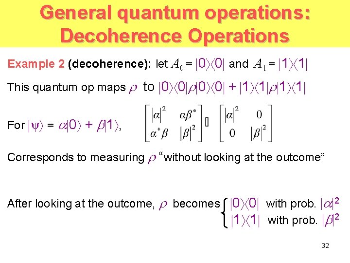
General quantum operations: Decoherence Operations Example 2 (decoherence): let A 0 = 0 0 and A 1 = 1 1 This quantum op maps to 0 0 + 1 1 For ψ = 0 + 1 , Corresponds to measuring “without looking at the outcome” After looking at the outcome, becomes 0 0 with prob. | |2 1 1 with prob. | |2 32

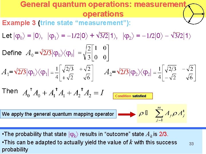
General quantum operations: measurement operations Example 3 (trine state “measurement”): Let 0 = 0 , 1 = 1/2 0 + 3/2 1 , 2 = 1/2 0 3/2 1 Define A 0 = 2/3 0 0 A 1= 2/3 1 1 A 2= 2/3 2 2 Then Condition satisfied We apply the general quantum mapping operator • The probability that state k results in “outcome” state Ak is 2/3. • This can be adapted to actually yield the value of k with this success probability 33

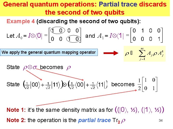
General quantum operations: Partial trace discards the second of two qubits Example 4 (discarding the second of two qubits): Let A 0 = I 0 and A 1 = I 1 We apply the general quantum mapping operator State becomes Note 1: it’s the same density matrix as for (( 0 , ½), ( 1 , ½)) Note 2: the operation is the partial trace Tr 2 34

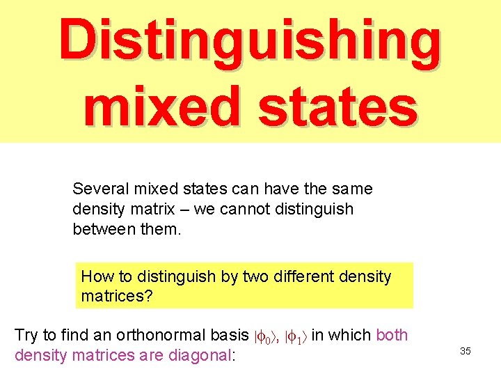
Distinguishing mixed states Several mixed states can have the same density matrix – we cannot distinguish between them. How to distinguish by two different density matrices? Try to find an orthonormal basis 0 , 1 in which both density matrices are diagonal: 35

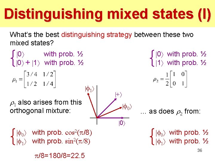
Distinguishing mixed states (I) What’s the best distinguishing strategy between these two mixed states? 0 with prob. ½ 1 with prob. ½ 0 with prob. ½ 0 + 1 with prob. ½ 1 1 also arises from this orthogonal mixture: + 0 … as does 2 from: 0 0 with prob. cos 2( /8) 1 with prob. sin 2( /8) /8=180/8=22. 5 0 with prob. ½ 1 with prob. ½ 36

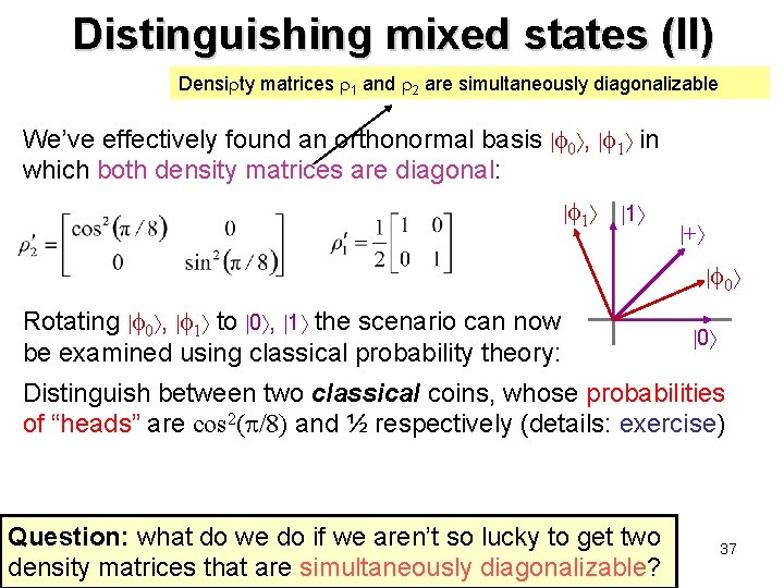
Distinguishing mixed states (II) Densi ty matrices 1 and 2 are simultaneously diagonalizable We’ve effectively found an orthonormal basis 0 , 1 in which both density matrices are diagonal: 1 1 + 0 Rotating 0 , 1 to 0 , 1 the scenario can now be examined using classical probability theory: 0 Distinguish between two classical coins, whose probabilities of “heads” are cos 2( /8) and ½ respectively (details: exercise) Question: what do we do if we aren’t so lucky to get two density matrices that are simultaneously diagonalizable? 37

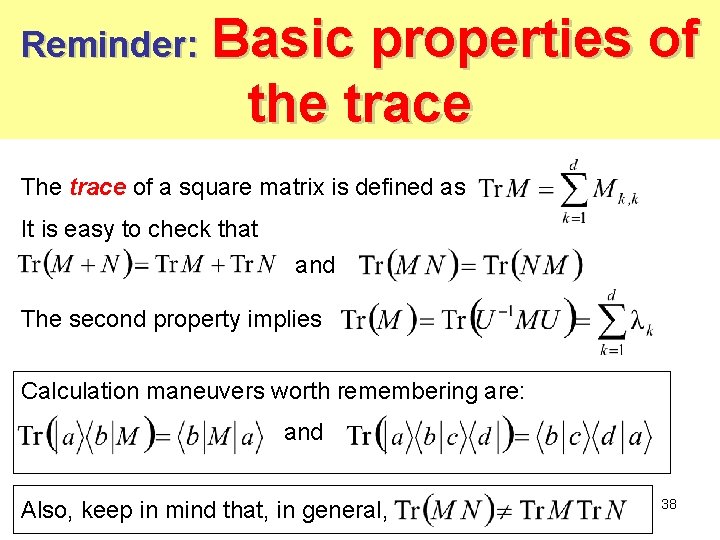
Reminder: Basic properties of the trace The trace of a square matrix is defined as It is easy to check that and The second property implies Calculation maneuvers worth remembering are: and Also, keep in mind that, in general, 38

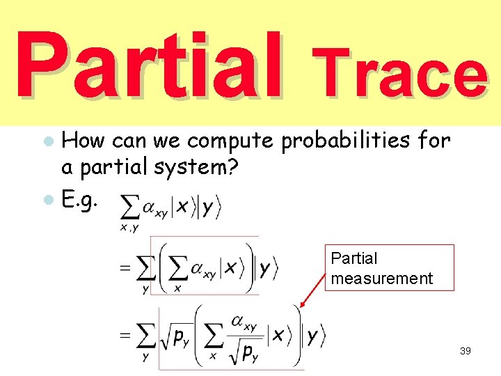
Partial Trace How can we compute probabilities for a partial system? l E. g. l Partial measurement 39

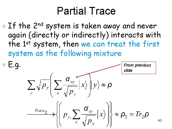
Partial Trace If the 2 nd system is taken away and never again (directly or indirectly) interacts with the 1 st system, then we can treat the first system as the following mixture From previous l E. g. l slide 40

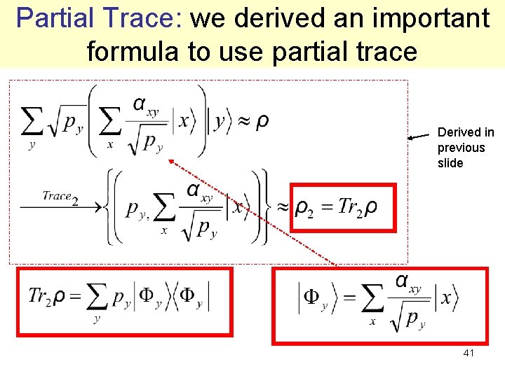
Partial Trace: we derived an important formula to use partial trace Derived in previous slide 41

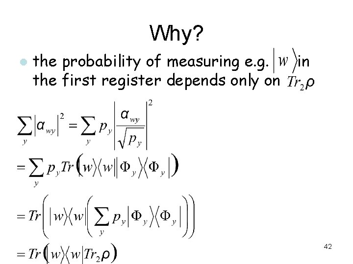
Why? l the probability of measuring e. g. the first register depends only on in 42

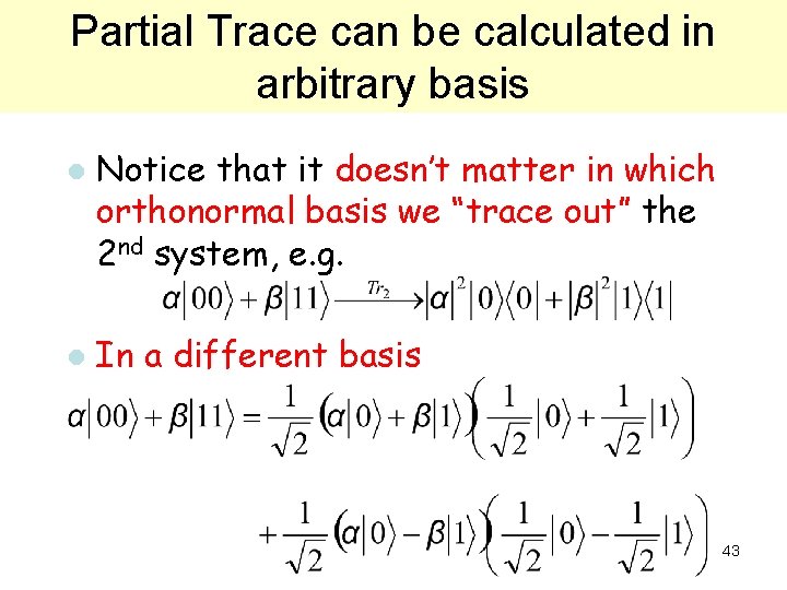
Partial Trace can be calculated in arbitrary basis l l Notice that it doesn’t matter in which orthonormal basis we “trace out” the 2 nd system, e. g. In a different basis 43

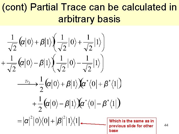
(cont) Partial Trace can be calculated in Partial Trace arbitrary basis Which is the same as in previous slide for other base 44

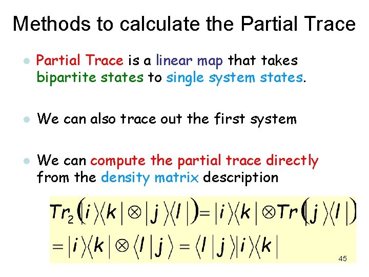
Methods to calculate the Partial Trace l l l Partial Trace is a linear map that takes bipartite states to single system states. We can also trace out the first system We can compute the partial trace directly from the density matrix description 45

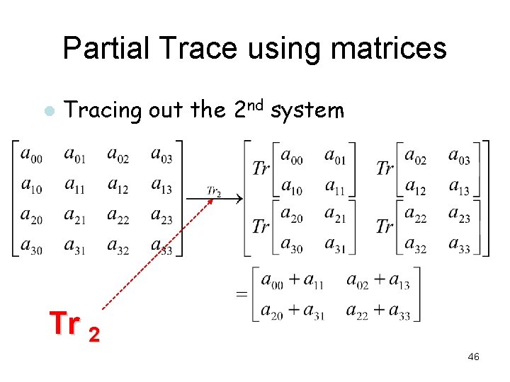
Partial Trace using matrices l Tracing out the 2 nd system Tr 2 46

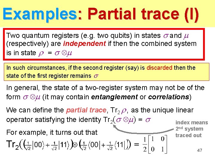
Examples: Partial trace (I) Two quantum registers (e. g. two qubits) in states and (respectively) are independent if then the combined system is in state = In such circumstances, if the second register (say) is discarded then the state of the first register remains In general, the state of a two-register system may not be of the form (it may contain entanglement or correlations) We can define the partial trace, Tr 2 , as the unique linear operator satisfying the identity Tr 2( ) = index means For example, it turns out that Tr 2( )= 2 nd system traced out 47

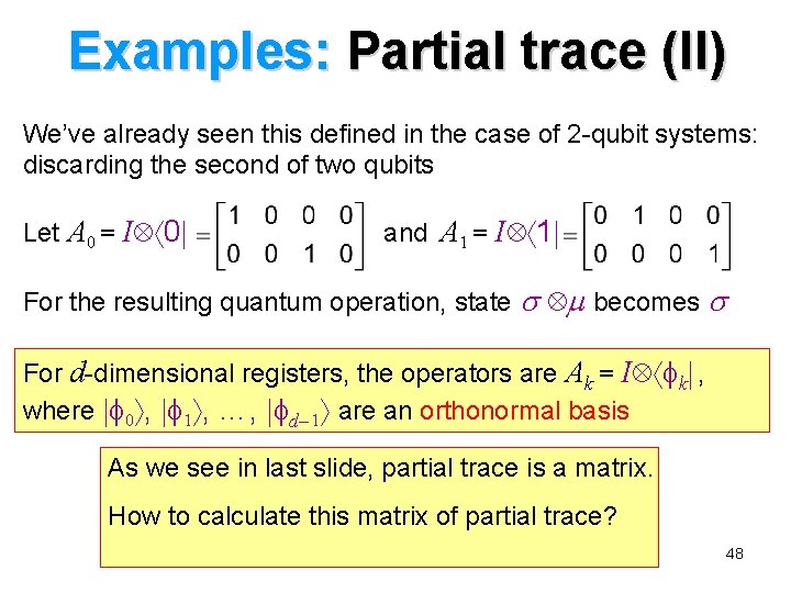
Examples: Partial trace (II) We’ve already seen this defined in the case of 2 -qubit systems: discarding the second of two qubits Let A 0 = I 0 and A 1 = I 1 For the resulting quantum operation, state becomes For d-dimensional registers, the operators are Ak = I k , where 0 , 1 , …, d 1 are an orthonormal basis As we see in last slide, partial trace is a matrix. How to calculate this matrix of partial trace? 48

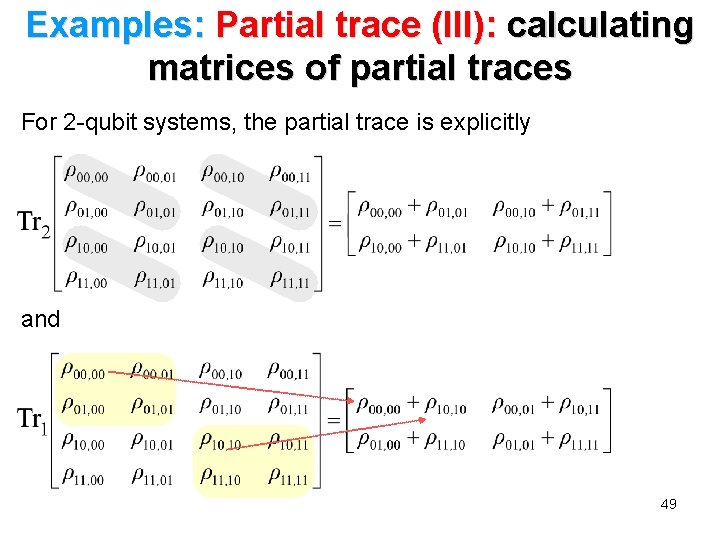
Examples: Partial trace (III): calculating matrices of partial traces For 2 -qubit systems, the partial trace is explicitly and 49

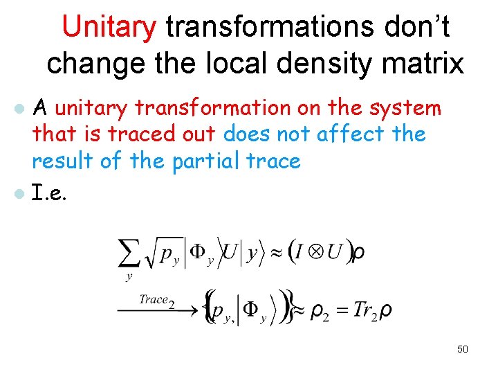
Unitary transformations don’t change the local density matrix A unitary transformation on the system that is traced out does not affect the result of the partial trace l I. e. l 50

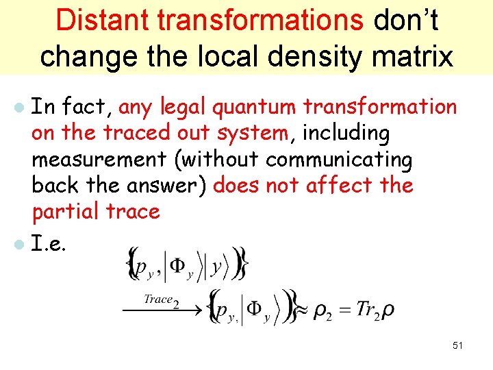
Distant transformations don’t change the local density matrix In fact, any legal quantum transformation on the traced out system, including measurement (without communicating back the answer) does not affect the partial trace l I. e. l 51

Why? ? l l Operations on the 2 nd system should not affect the statistics of any outcomes of measurements on the first system Otherwise a party in control of the 2 nd system could instantaneously communicate information to a party controlling the 1 st system. 52

Principle of implicit measurement l l If some qubits in a computation are never used again, you can assume (if you like) that they have been measured (and the result ignored) The “reduced density matrix” of the remaining qubits is the same 53

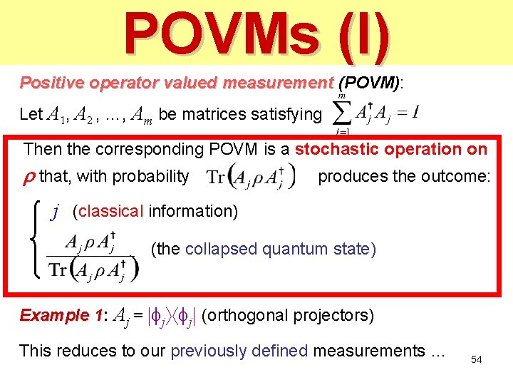
POVMs (I) Positive operator valued measurement (POVM): Let A 1, A 2 , …, Am be matrices satisfying Then the corresponding POVM is a stochastic operation on that, with probability produces the outcome: j (classical information) (the collapsed quantum state) Example 1: 1 Aj = j j (orthogonal projectors) This reduces to our previously defined measurements … 54

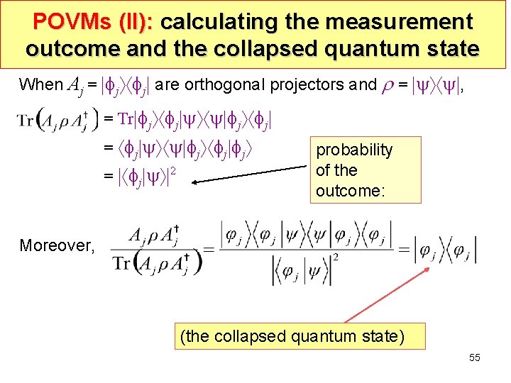
POVMs (II): calculating the measurement outcome and the collapsed quantum state When Aj = j j are orthogonal projectors and = , = Tr j j = j j j j = j 2 probability of the outcome: Moreover, (the collapsed quantum state) 55

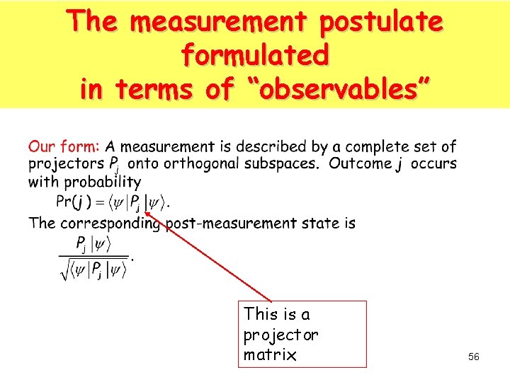
The measurement postulate formulated in terms of “observables” This is a projector matrix 56

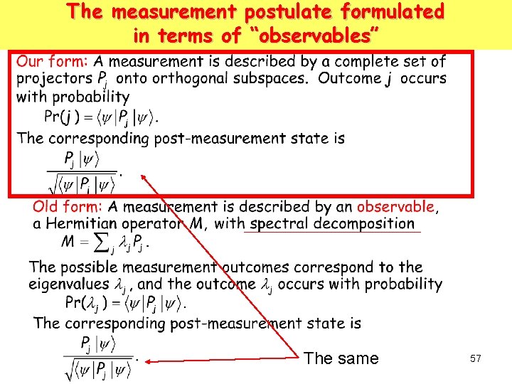
The measurement postulate formulated in terms of “observables” The same 57

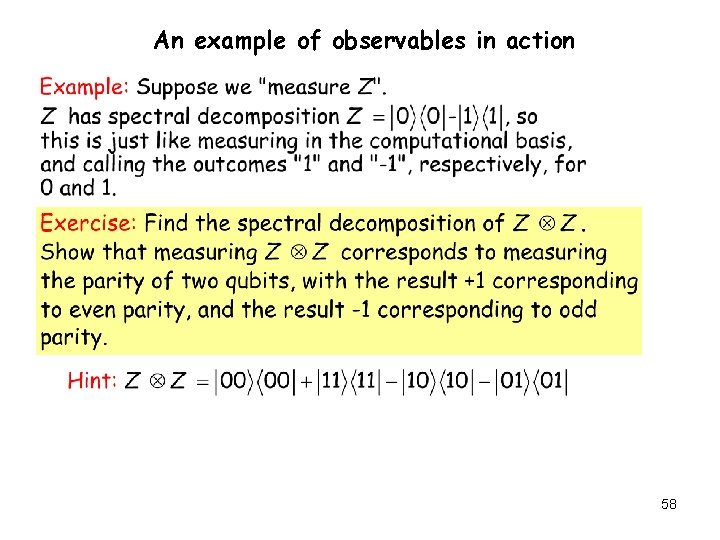
An example of observables in action 58

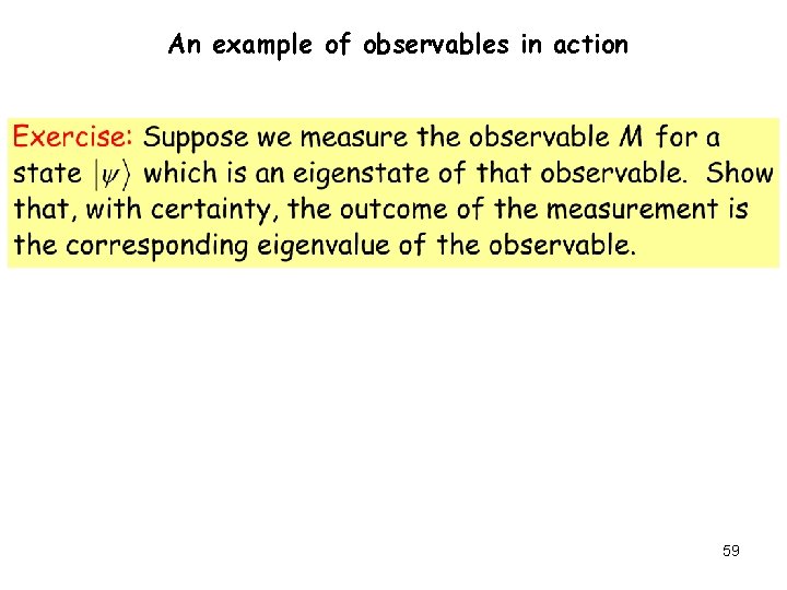
An example of observables in action 59

What can be measured in quantum mechanics? Computer science can inspire fundamental questions about physics. We may take an “informatic” approach to physics. (Compare the physical approach to information. ) Problem: What measurements can be performed in quantum mechanics? 60

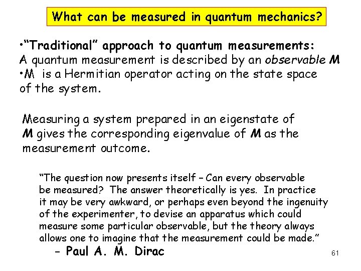
What can be measured in quantum mechanics? • “Traditional” approach to quantum measurements: A quantum measurement is described by an observable M • M is a Hermitian operator acting on the state space of the system. Measuring a system prepared in an eigenstate of M gives the corresponding eigenvalue of M as the measurement outcome. “The question now presents itself – Can every observable be measured? The answer theoretically is yes. In practice it may be very awkward, or perhaps even beyond the ingenuity of the experimenter, to devise an apparatus which could measure some particular observable, but theory always allows one to imagine that the measurement could be made. ” - Paul A. M. Dirac 61

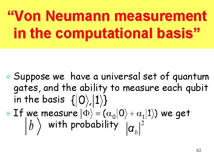
“Von Neumann measurement in the computational basis” Suppose we have a universal set of quantum gates, and the ability to measure each qubit in the basis l If we measure we get with probability l 62

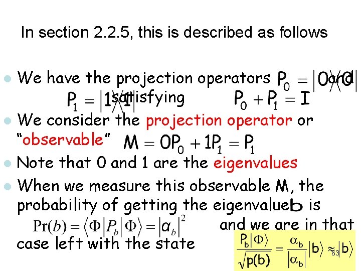
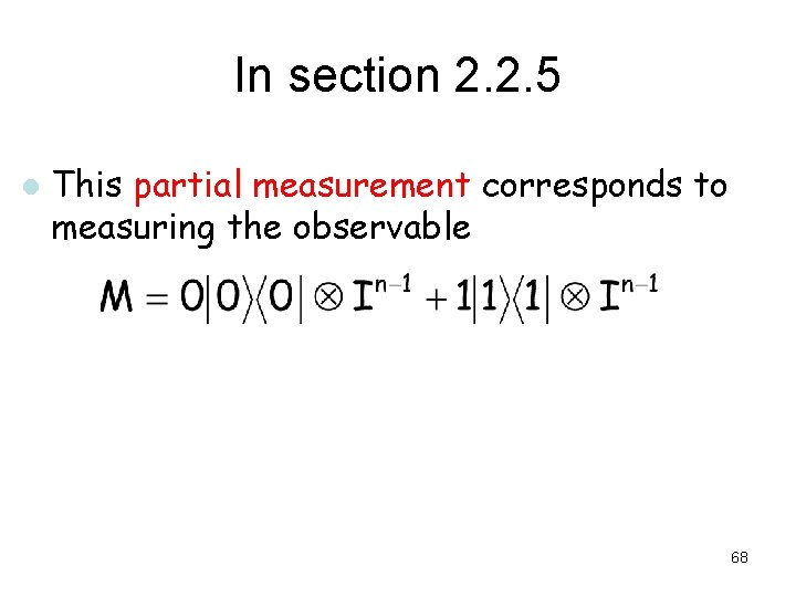
In section 2. 2. 5, this is described as follows We have the projection operators and satisfying l We consider the projection operator or “observable” l Note that 0 and 1 are the eigenvalues l When we measure this observable M, the probability of getting the eigenvalue is and we are in that case left with the state 63 l

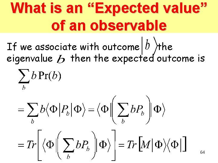
What is an “Expected value” of an observable If we associate with outcome the eigenvalue then the expected outcome is 64

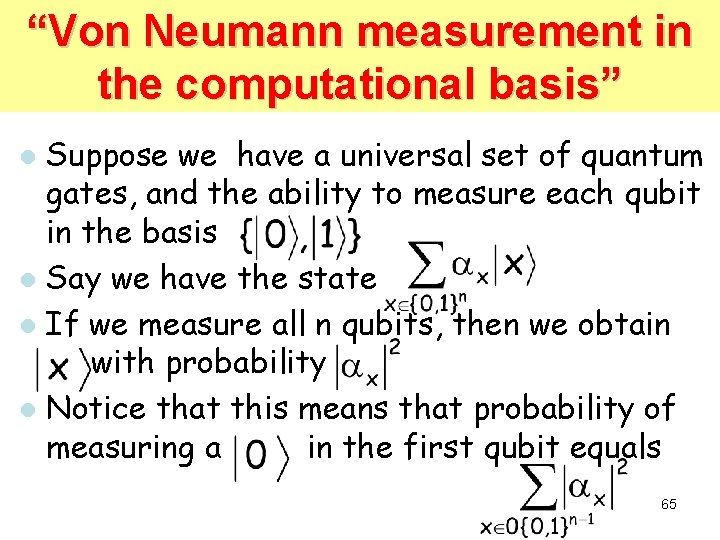
“Von Neumann measurement in the computational basis” Suppose we have a universal set of quantum gates, and the ability to measure each qubit in the basis l Say we have the state l If we measure all n qubits, then we obtain with probability l Notice that this means that probability of measuring a in the first qubit equals l 65

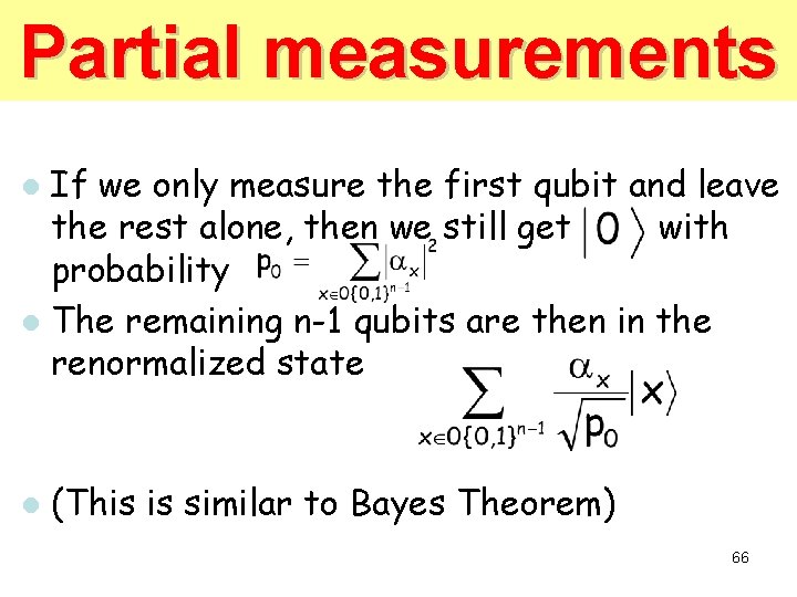
Partial measurements If we only measure the first qubit and leave the rest alone, then we still get with probability l The remaining n-1 qubits are then in the renormalized state l l (This is similar to Bayes Theorem) 66

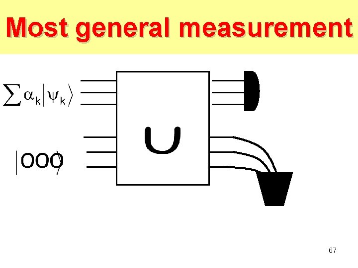
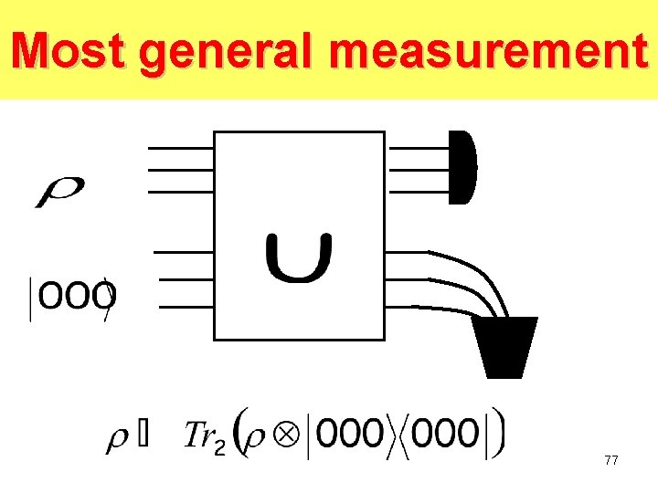
Most general measurement 67

In section 2. 2. 5 l This partial measurement corresponds to measuring the observable 68

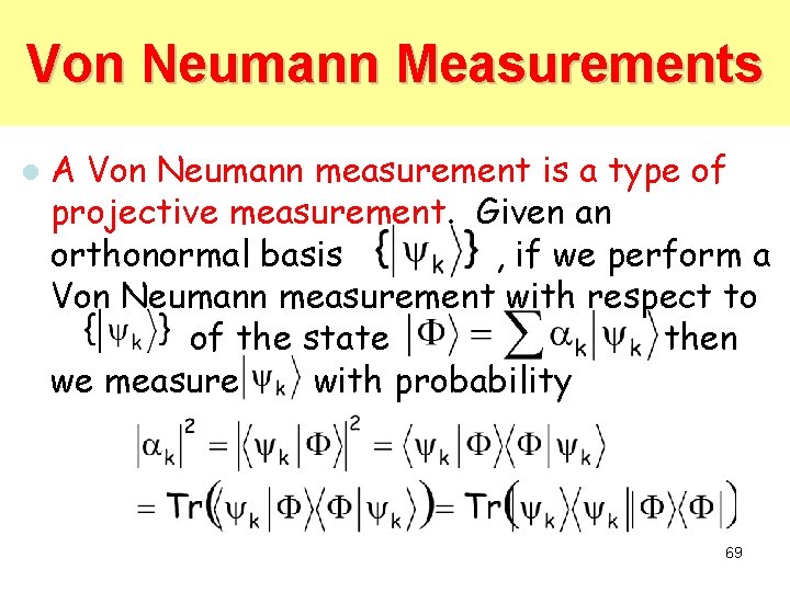
Von Neumann Measurements l A Von Neumann measurement is a type of projective measurement. Given an orthonormal basis , if we perform a Von Neumann measurement with respect to of the state then we measure with probability 69

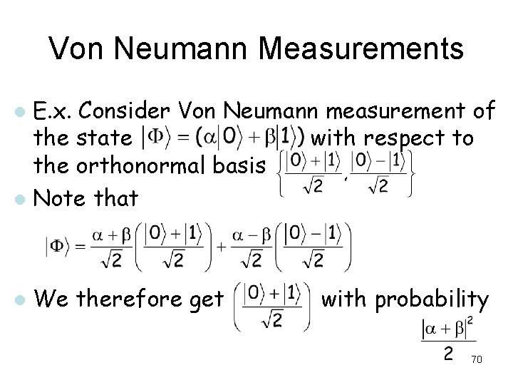
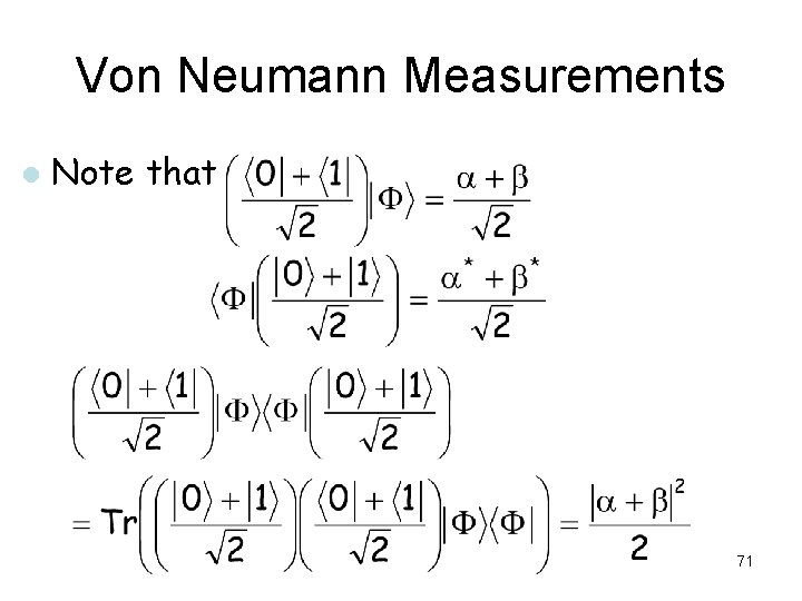
Von Neumann Measurements E. x. Consider Von Neumann measurement of the state with respect to the orthonormal basis l Note that l l We therefore get with probability 70

Von Neumann Measurements l Note that 71

How do we implement Von Neumann measurements? l If we have access to a universal set of gates and bit-wise measurements in the computational basis, we can implement Von Neumann measurements with respect to an arbitrary orthonormal basis as follows. 72

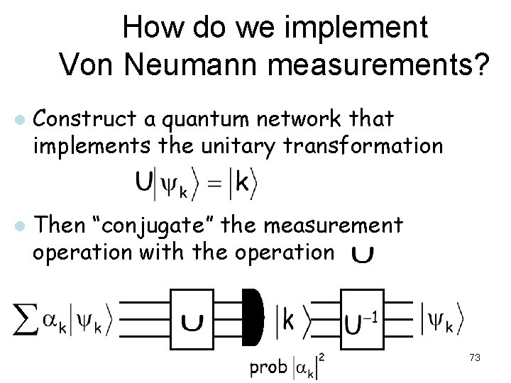
How do we implement Von Neumann measurements? l l Construct a quantum network that implements the unitary transformation Then “conjugate” the measurement operation with the operation 73

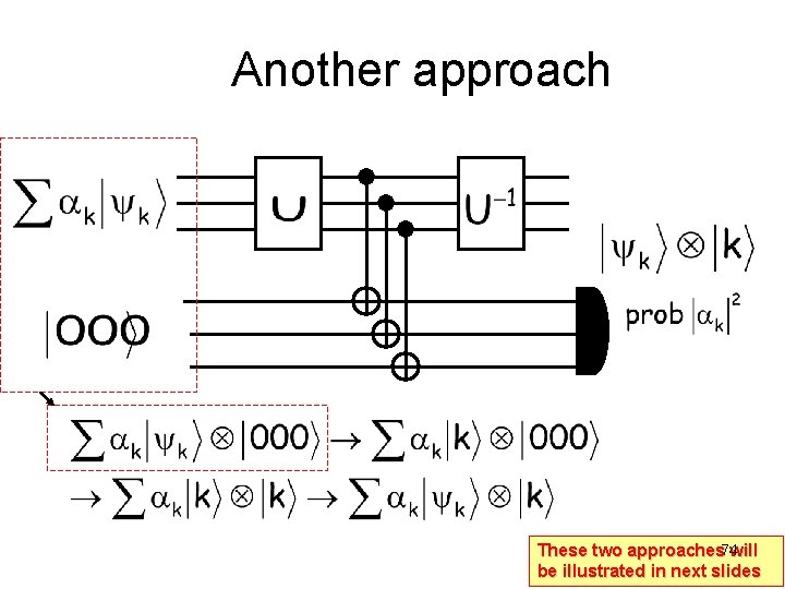
Another approach These two approaches 74 will be illustrated in next slides

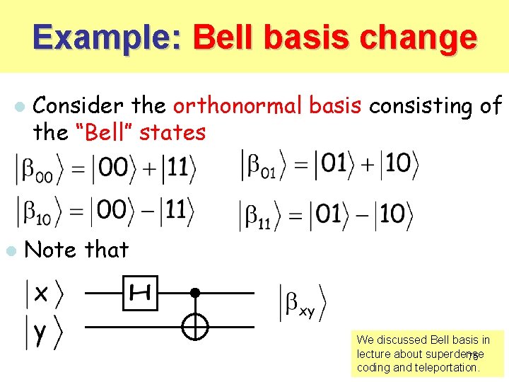
Example: Bell basis change l l Consider the orthonormal basis consisting of the “Bell” states Note that We discussed Bell basis in lecture about superdense 75 coding and teleportation.

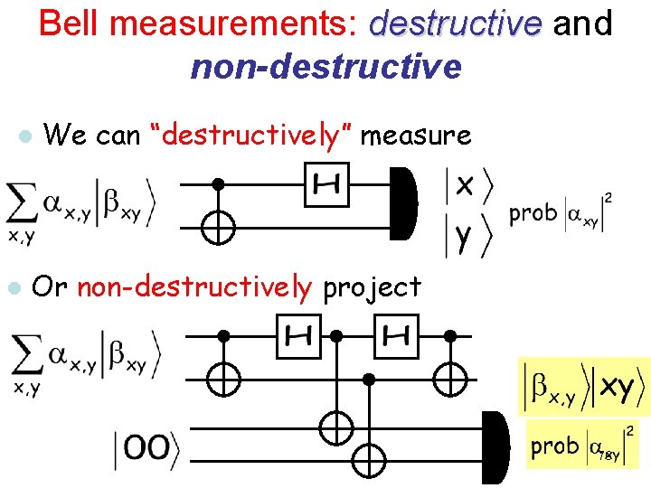
Bell measurements: destructive and non-destructive l l We can “destructively” measure Or non-destructively project 76

Most general measurement 77

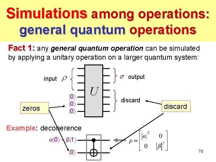
Simulations among operations: general quantum operations Fact 1: any general quantum operation can be simulated by applying a unitary operation on a larger quantum system: input zeros 0 0 0 U output discard Example: decoherence 0 + 1 0 78

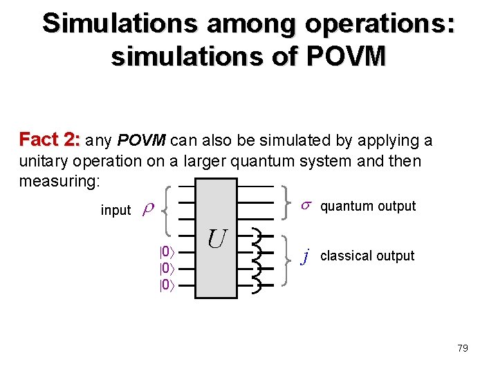
Simulations among operations: simulations of POVM Fact 2: any POVM can also be simulated by applying a unitary operation on a larger quantum system and then measuring: input 0 0 0 U quantum output j classical output 79

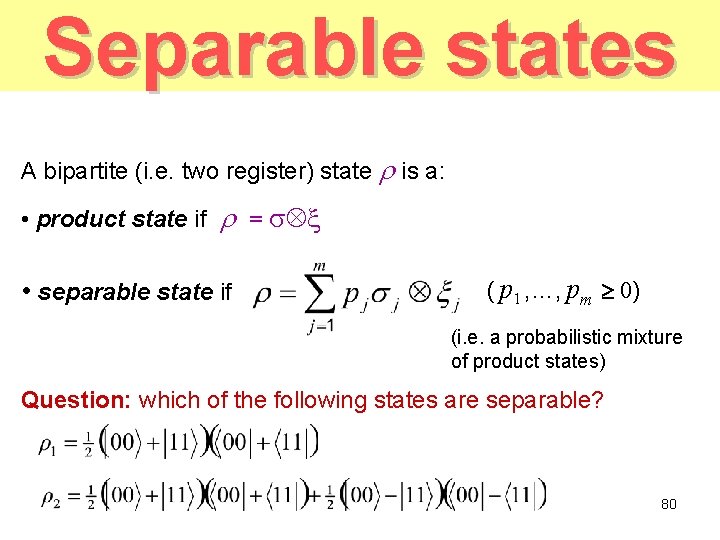
Separable states A bipartite (i. e. two register) state is a: • product state if = • separable state if ( p 1 , …, pm 0) (i. e. a probabilistic mixture of product states) Question: which of the following states are separable? 80

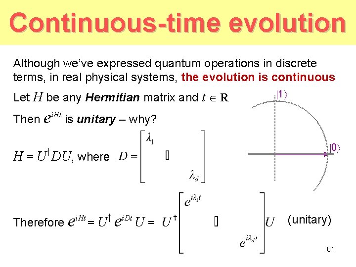
Continuous-time evolution Although we’ve expressed quantum operations in discrete terms, in real physical systems, the evolution is continuous Let H be any Hermitian matrix and t R 1 Then ei. Ht is unitary – why? 0 † H = U DU, where Therefore e i. Ht =U † ei. Dt U = (unitary) 81

Partially covered in 2007: • • • Density matrices and indistinguishable states Taxonomy of normal operators General Quantum Operations Distinguishing states Partial trace POVM Simulations of operators Separable states Continuous time evolution 82