Econometrics Chengyuan Yin School of Mathematics Econometrics 17

Econometrics Chengyuan Yin School of Mathematics

Econometrics 17. Linear Models for Panel Data

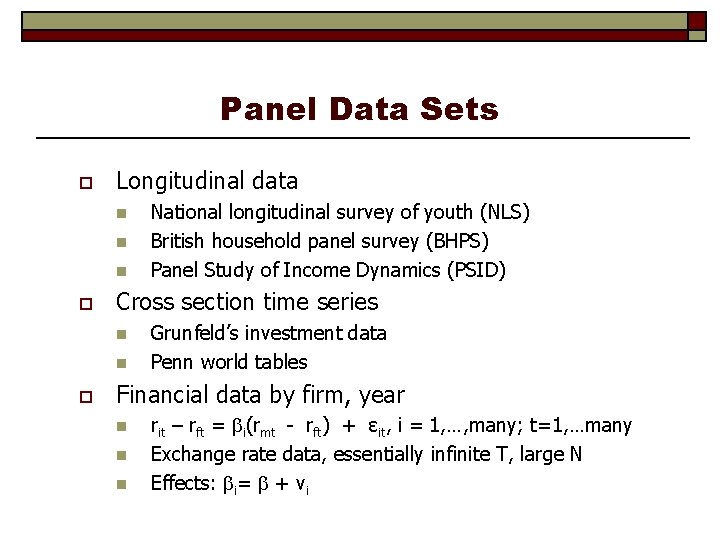
Panel Data Sets o Longitudinal data n n n o Cross section time series n n o National longitudinal survey of youth (NLS) British household panel survey (BHPS) Panel Study of Income Dynamics (PSID) Grunfeld’s investment data Penn world tables Financial data by firm, year n n n rit – rft = i(rmt - rft) + εit, i = 1, …, many; t=1, …many Exchange rate data, essentially infinite T, large N Effects: i= + vi

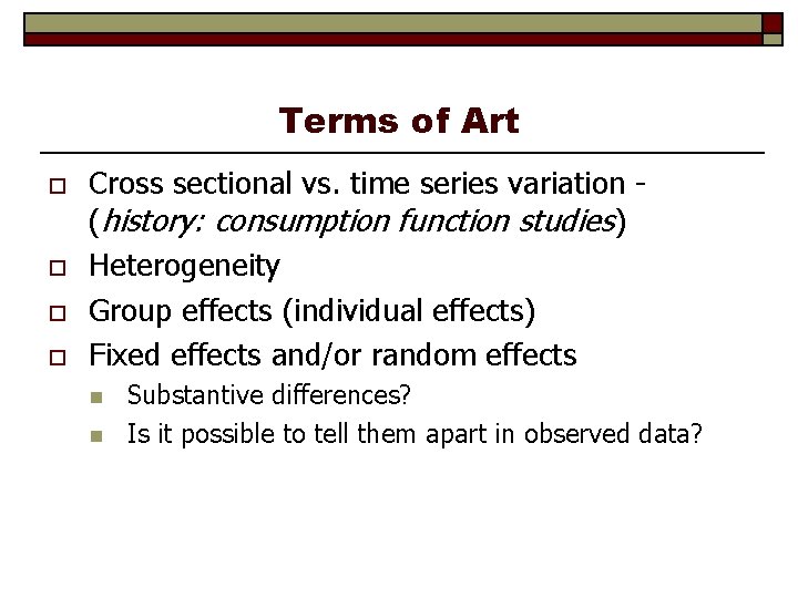
Terms of Art o o Cross sectional vs. time series variation (history: consumption function studies) Heterogeneity Group effects (individual effects) Fixed effects and/or random effects n n Substantive differences? Is it possible to tell them apart in observed data?

Panel Data o Rotating panels: Spanish household survey n n o Spanish income study (http: //www. cemfi. es/~albarran/0008 r. pdf) Efficiency analysis: “Efficiency measurement in rotating panel data, ” Heshmati, A, Applied Economics, 30, 1998, pp. 919 -930 Hierarchical (nested) data sets: Student outcome, by year, district, school, teacher

Nested Panel Data o Antweiler, W. , Nested Random Effects…” Journal of Econometrics, 101, 2001, 295 -313

Balanced and Unbalanced Panels o o Distinction A notation to help with mechanics zi, t, i = 1, …, N; t = 1, …, Ti o The role of the assumption n Mathematical and notational convenience: o o n Balanced, NT Unbalanced: Is the fixed Ti assumption ever necessary? SUR models.

Benefits of Panel Data o o Time and individual variation in behavior unobservable in cross sections or aggregate time series Observable and unobservable individual heterogeneity Rich hierarchical structures Dynamics in economic behavior

Fixed and Random Effects o Unobserved individual effects in regression: E[yit | xit, ci] n Notation: n o Linear specification: n Fixed Effects: E[ci | Xi ] = g(Xi); effects are correlated with included variables. Common: Cov[xit, ci] ≠ 0 n Random Effects: E[ci | Xi ] = μ; effects are uncorrelated with included variables. If Xi contains a constant term, μ=0 WLOG. Common: Cov[xit, ci] =0, but E[ci | Xi ] = μ is needed for the full model

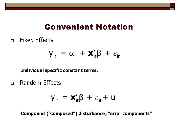
Convenient Notation o Fixed Effects Individual specific constant terms. o Random Effects Compound (“composed”) disturbance; “error components”

Assumptions for Asymptotics o o Convergence of moments involving cross section Xi. N increasing, T or Ti assumed fixed. n n n o o o “Fixed T asymptotics” (see text, p. 196) Time series characteristics are not relevant (may be nonstationary) If T is also growing, need to treat as multivariate time series. Ranks of matrices. X must have full column rank. (Xi may not, if Ti < K. ) Strict exogeneity and dynamics. If xit contains yi, t-1 then xit cannot be strictly exogenous. Xit will be correlated with the unobservables in period t-1. (To be revisited later. ) Empirical characteristics of microeconomic data

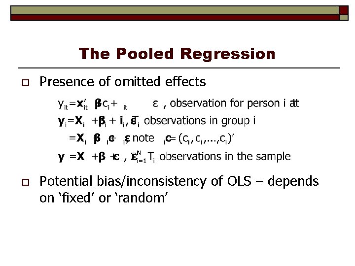
The Pooled Regression o o Presence of omitted effects Potential bias/inconsistency of OLS – depends on ‘fixed’ or ‘random’

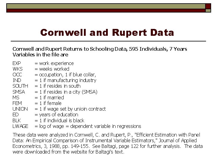
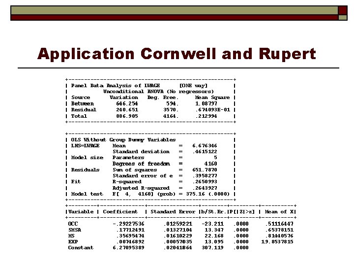
Cornwell and Rupert Data Cornwell and Rupert Returns to Schooling Data, 595 Individuals, 7 Years Variables in the file are EXP WKS OCC IND SOUTH SMSA MS FEM UNION ED BLK LWAGE = = = work experience weeks worked occupation, 1 if blue collar, 1 if manufacturing industry 1 if resides in south 1 if resides in a city (SMSA) 1 if married 1 if female 1 if wage set by unioin contract years of education 1 if individual is black log of wage = dependent variable in regressions These data were analyzed in Cornwell, C. and Rupert, P. , "Efficient Estimation with Panel Data: An Empirical Comparison of Instrumental Variable Estimators, " Journal of Applied Econometrics, 3, 1988, pp. 149 -155. See Baltagi, page 122 for further analysis. The data were downloaded from the website for Baltagi's text.

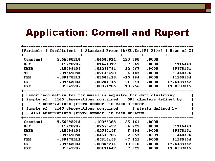
Application: Cornell and Rupert

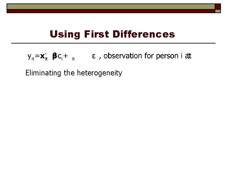
Using First Differences Eliminating the heterogeneity

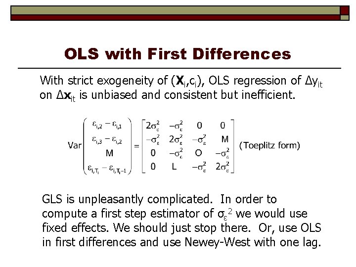
OLS with First Differences With strict exogeneity of (Xi, ci), OLS regression of Δyit on Δxit is unbiased and consistent but inefficient. GLS is unpleasantly complicated. In order to compute a first step estimator of σε 2 we would use fixed effects. We should just stop there. Or, use OLS in first differences and use Newey-West with one lag.

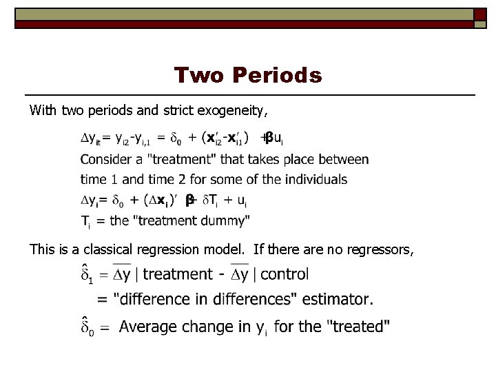
Two Periods With two periods and strict exogeneity, This is a classical regression model. If there are no regressors,

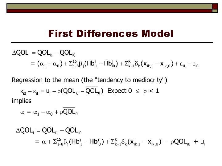
Application of a Two Period Model o o “Hemoglobin and Quality of Life in Cancer Patients with Anemia, ” Finkelstein (MIT), Berndt (MIT), Greene (NYU), Cremieux (Univ. of Quebec) 1998 With Ortho Biotech – seeking to change labeling of already approved drug ‘erythropoetin. ’ r -Hu. EPO

QOL Study o Quality of life study n n o o yit = self administered quality of life survey, scale = 0, …, 100 xit = hemoglobin level, other covariates n n o Treatment effects model (hemoglobin level) Background – r-Hu. EPO treatment to affect Hg level Important statistical issues n n o i = 1, … 1200+ clinically anemic cancer patients undergoing chemotherapy, treated with transfusions and/or r-Hu. EPO t = 0 at baseline, 1 at exit. (interperiod survey by some patients was not used) Unobservable individual effects The placebo effect Attrition – sample selection FDA mistrust of “community based” – not clinical trial based statistical evidence Objective – when to administer treatment for maximum marginal benefit

Regression-Treatment Effects Model

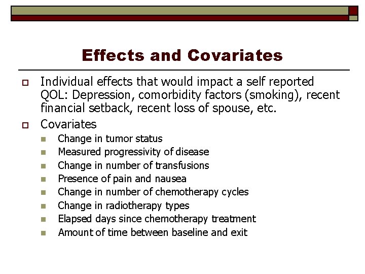
Effects and Covariates o o Individual effects that would impact a self reported QOL: Depression, comorbidity factors (smoking), recent financial setback, recent loss of spouse, etc. Covariates n n n n Change in tumor status Measured progressivity of disease Change in number of transfusions Presence of pain and nausea Change in number of chemotherapy cycles Change in radiotherapy types Elapsed days since chemotherapy treatment Amount of time between baseline and exit

First Differences Model

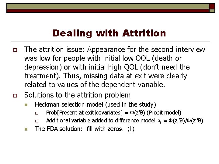
Dealing with Attrition o o The attrition issue: Appearance for the second interview was low for people with initial low QOL (death or depression) or with initial high QOL (don’t need the treatment). Thus, missing data at exit were clearly related to values of the dependent variable. Solutions to the attrition problem n Heckman selection model (used in the study) o o n Prob[Present at exit|covariates] = Φ(z’θ) (Probit model) Additional variable added to difference model i = Φ(zi’θ)/Φ(zi’θ) The FDA solution: fill with zeros. (!)

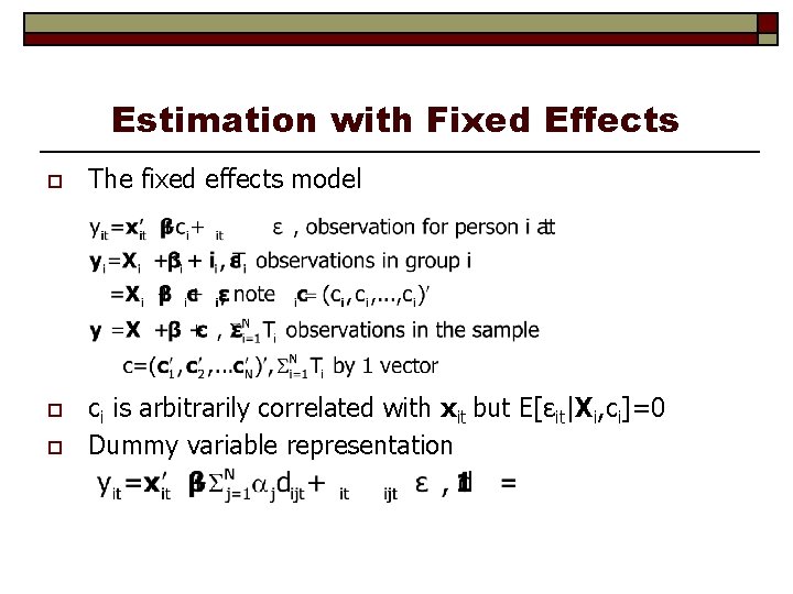
Estimation with Fixed Effects o The fixed effects model o ci is arbitrarily correlated with xit but E[εit|Xi, ci]=0 Dummy variable representation o

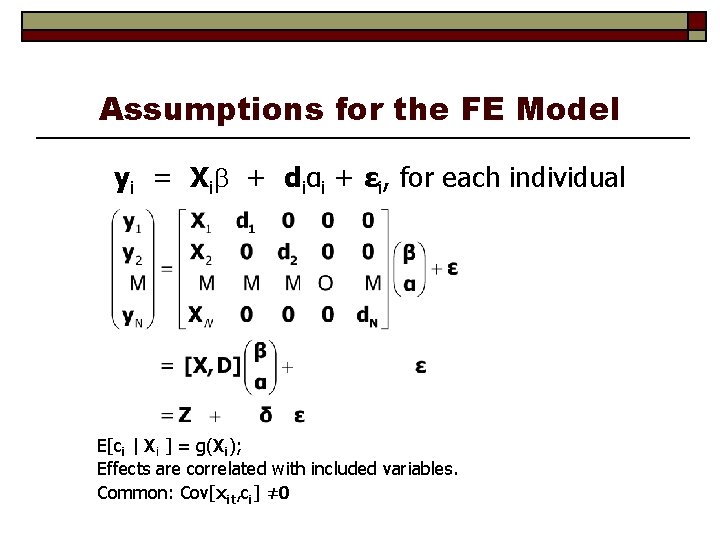
Assumptions for the FE Model yi = Xi + diαi + εi, for each individual E[ci | Xi ] = g(Xi); Effects are correlated with included variables. Common: Cov[xit, ci] ≠ 0

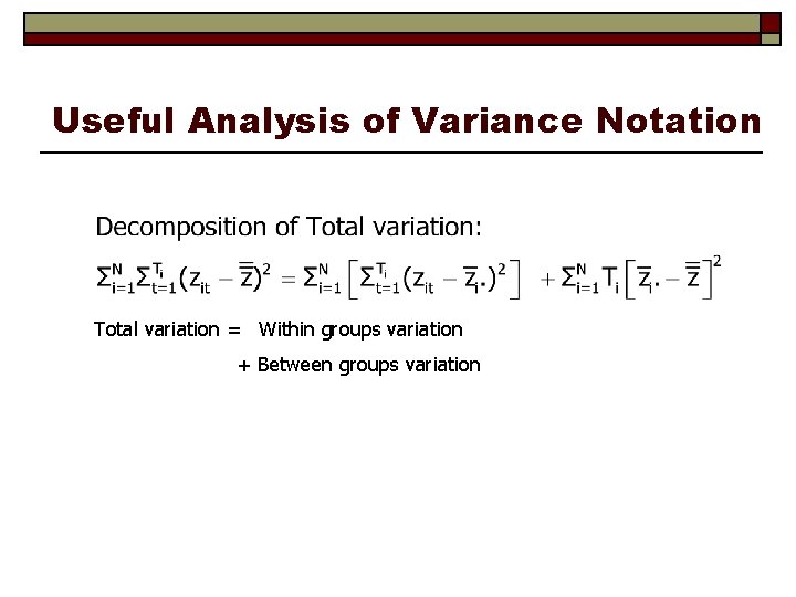
Useful Analysis of Variance Notation Total variation = Within groups variation + Between groups variation

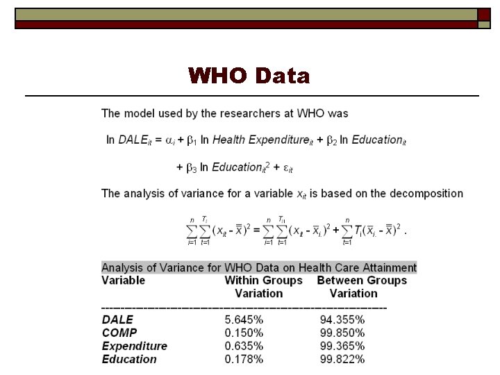
WHO Data

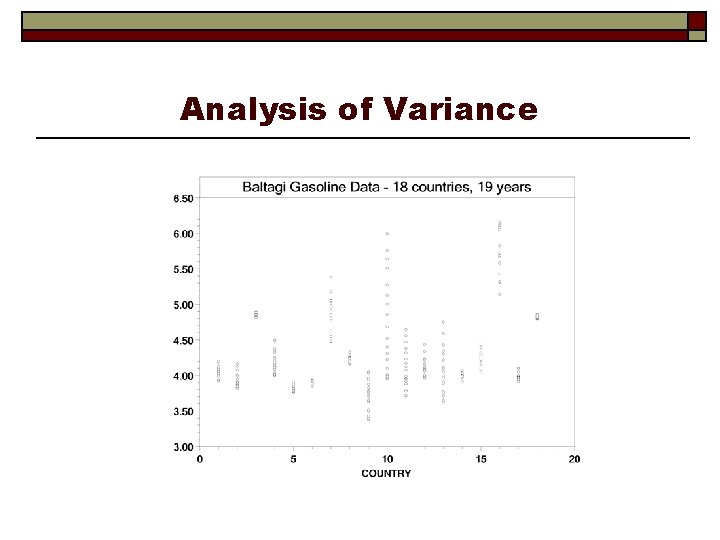
Baltagi and Griffin’s Gasoline Data World Gasoline Demand Data, 18 OECD Countries, 19 years Variables in the file are COUNTRY = name of country YEAR = year, 1960 -1978 LGASPCAR = log of consumption per car LINCOMEP = log of per capita income LRPMG = log of real price of gasoline LCARPCAP = log of per capita number of cars See Baltagi (2001, p. 24) for analysis of these data. The article on which the analysis is based is Baltagi, B. and Griffin, J. , "Gasolne Demand in the OECD: An Application of Pooling and Testing Procedures, " European Economic Review, 22, 1983, pp. 117 -137. The data were downloaded from the website for Baltagi's text.

Analysis of Variance

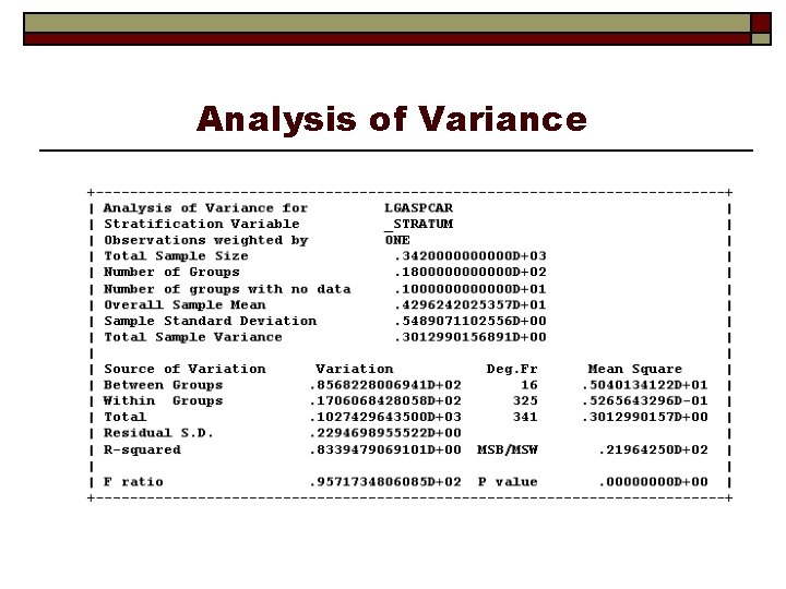
Analysis of Variance

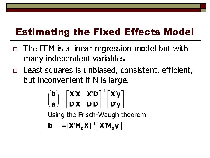
Estimating the Fixed Effects Model o o The FEM is a linear regression model but with many independent variables Least squares is unbiased, consistent, efficient, but inconvenient if N is large.

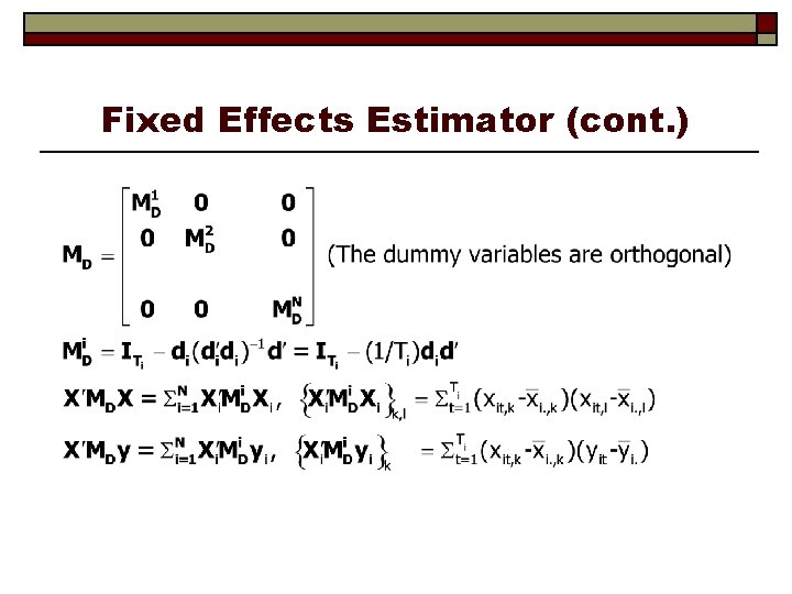
Fixed Effects Estimator (cont. )

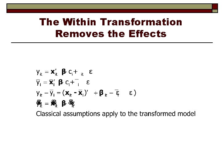
The Within Transformation Removes the Effects

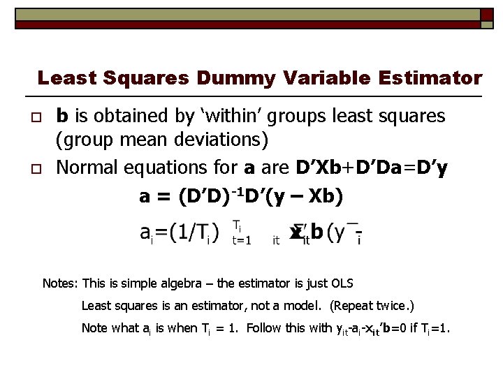
Least Squares Dummy Variable Estimator o o b is obtained by ‘within’ groups least squares (group mean deviations) Normal equations for a are D’Xb+D’Da=D’y a = (D’D)-1 D’(y – Xb) Notes: This is simple algebra – the estimator is just OLS Least squares is an estimator, not a model. (Repeat twice. ) Note what ai is when Ti = 1. Follow this with yit-ai-xit’b=0 if Ti=1.

Inference About OLS o o o Assume strict exogeneity: Cov[εit, (xjs, cj)]=0. Every disturbance in every period for each person is uncorrelated with variables and effects for every person and across periods. Now, it’s just least squares in a classical linear regression model. Asy. Var[b] =

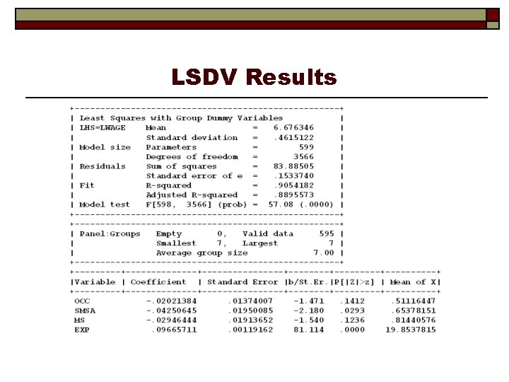
Application Cornwell and Rupert

LSDV Results

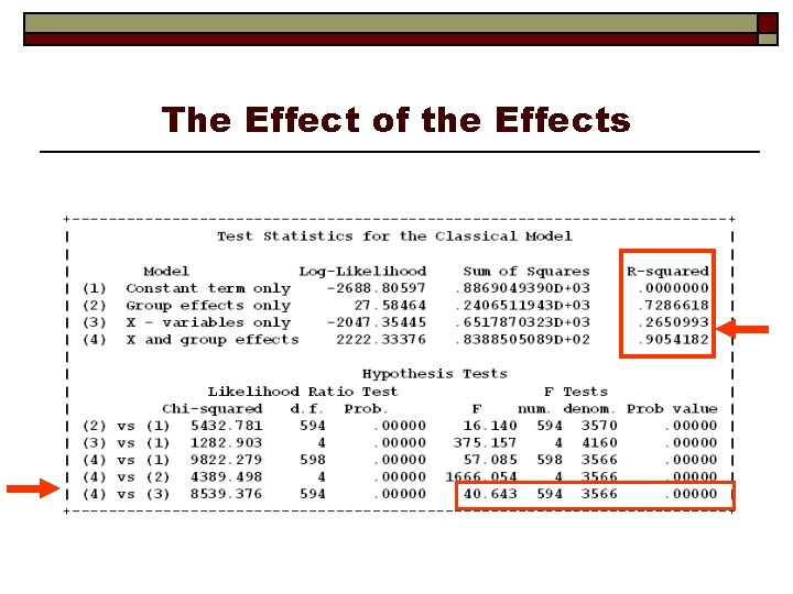
The Effect of the Effects

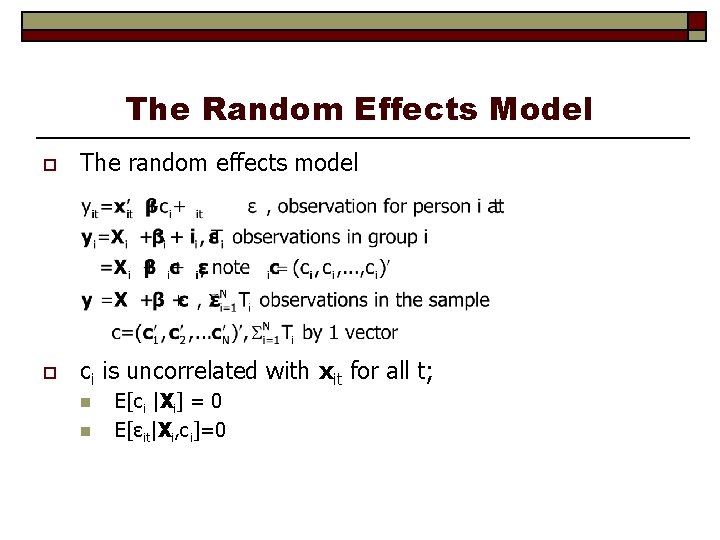
The Random Effects Model o The random effects model o ci is uncorrelated with xit for all t; n n E[ci |Xi] = 0 E[εit|Xi, ci]=0

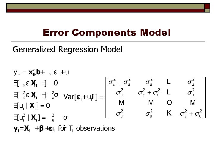
Error Components Model Generalized Regression Model

Notation

Notation

Convergence of Moments

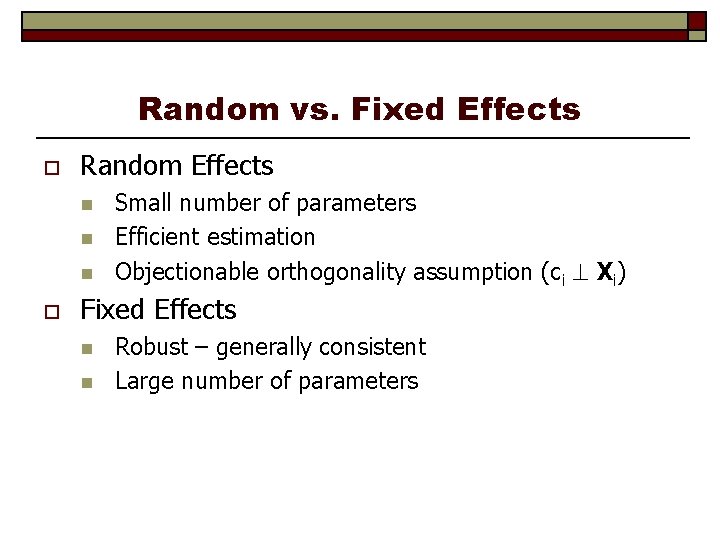
Random vs. Fixed Effects o Random Effects n n n o Small number of parameters Efficient estimation Objectionable orthogonality assumption (ci Xi) Fixed Effects n n Robust – generally consistent Large number of parameters

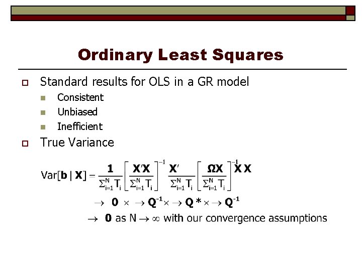
Ordinary Least Squares o Standard results for OLS in a GR model n n n o Consistent Unbiased Inefficient True Variance

Estimating the Variance for OLS

Mechanics

Cornwell and Rupert Data Cornwell and Rupert Returns to Schooling Data, 595 Individuals, 7 Years Variables in the file are EXP WKS OCC IND SOUTH SMSA MS FEM UNION ED BLK LWAGE = = = work experience, EXPSQ = EXP 2 weeks worked occupation, 1 if blue collar, 1 if manufacturing industry 1 if resides in south 1 if resides in a city (SMSA) 1 if married 1 if female 1 if wage set by unioin contract years of education 1 if individual is black log of wage = dependent variable in regressions These data were analyzed in Cornwell, C. and Rupert, P. , "Efficient Estimation with Panel Data: An Empirical Comparison of Instrumental Variable Estimators, " Journal of Applied Econometrics, 3, 1988, pp. 149 -155. See Baltagi, page 122 for further analysis. The data were downloaded from the website for Baltagi's text.

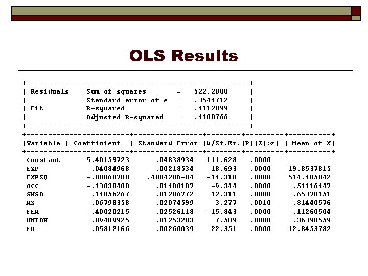
OLS Results +--------------------------+ | Residuals Sum of squares = 522. 2008 | | Standard error of e =. 3544712 | | Fit R-squared =. 4112099 | | Adjusted R-squared =. 4100766 | +--------------------------+ +--------------+--------+---------+-----+ |Variable | Coefficient | Standard Error |b/St. Er. |P[|Z|>z] | Mean of X| +--------------+--------+---------+-----+ Constant 5. 40159723. 04838934 111. 628. 0000 EXP. 04084968. 00218534 18. 693. 0000 19. 8537815 EXPSQ -. 00068788. 480428 D-04 -14. 318. 0000 514. 405042 OCC -. 13830480. 01480107 -9. 344. 0000. 51116447 SMSA. 14856267. 01206772 12. 311. 0000. 65378151 MS. 06798358. 02074599 3. 277. 0010. 81440576 FEM -. 40020215. 02526118 -15. 843. 0000. 11260504 UNION. 09409925. 01253203 7. 509. 0000. 36398559 ED. 05812166. 00260039 22. 351. 0000 12. 8453782

Alternative Variance Estimators +--------------+--------+---------+ |Variable | Coefficient | Standard Error |b/St. Er. |P[|Z|>z] | +--------------+--------+---------+ Constant 5. 40159723. 04838934 111. 628. 0000 EXP. 04084968. 00218534 18. 693. 0000 EXPSQ -. 00068788. 480428 D-04 -14. 318. 0000 OCC -. 13830480. 01480107 -9. 344. 0000 SMSA. 14856267. 01206772 12. 311. 0000 MS. 06798358. 02074599 3. 277. 0010 FEM -. 40020215. 02526118 -15. 843. 0000 UNION. 09409925. 01253203 7. 509. 0000 ED. 05812166. 00260039 22. 351. 0000 Robust Constant 5. 40159723. 10156038 53. 186. 0000 EXP. 04084968. 00432272 9. 450. 0000 EXPSQ -. 00068788. 983981 D-04 -6. 991. 0000 OCC -. 13830480. 02772631 -4. 988. 0000 SMSA. 14856267. 02423668 6. 130. 0000 MS. 06798358. 04382220 1. 551. 1208 FEM -. 40020215. 04961926 -8. 065. 0000 UNION. 09409925. 02422669 3. 884. 0001 ED. 05812166. 00555697 10. 459. 0000

Generalized Least Squares

GLS (cont. )

Estimators for the Variances

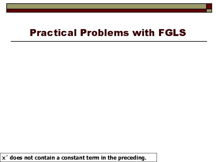
Feasible GLS x´ does not contain a constant term in the preceding.

Practical Problems with FGLS x´ does not contain a constant term in the preceding.

Computing Variance Estimators

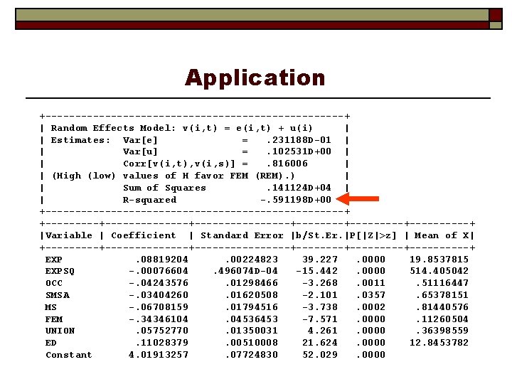
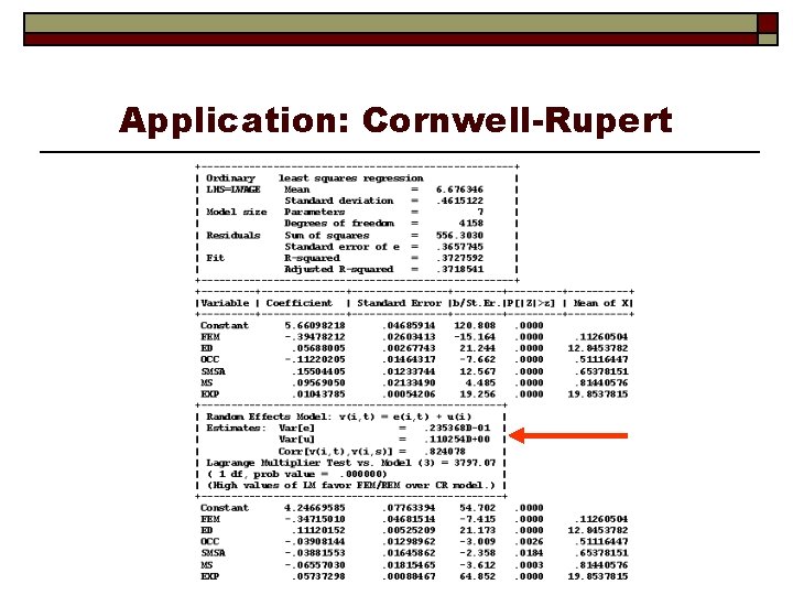
Application +-------------------------+ | Random Effects Model: v(i, t) = e(i, t) + u(i) | | Estimates: Var[e] =. 231188 D-01 | | Var[u] =. 102531 D+00 | | Corr[v(i, t), v(i, s)] =. 816006 | | (High (low) values of H favor FEM (REM). ) | | Sum of Squares. 141124 D+04 | | R-squared -. 591198 D+00 | +-------------------------+ +--------------+--------+---------+-----+ |Variable | Coefficient | Standard Error |b/St. Er. |P[|Z|>z] | Mean of X| +--------------+--------+---------+-----+ EXP. 08819204. 00224823 39. 227. 0000 19. 8537815 EXPSQ -. 00076604. 496074 D-04 -15. 442. 0000 514. 405042 OCC -. 04243576. 01298466 -3. 268. 0011. 51116447 SMSA -. 03404260. 01620508 -2. 101. 0357. 65378151 MS -. 06708159. 01794516 -3. 738. 0002. 81440576 FEM -. 34346104. 04536453 -7. 571. 0000. 11260504 UNION. 05752770. 01350031 4. 261. 0000. 36398559 ED. 11028379. 00510008 21. 624. 0000 12. 8453782 Constant 4. 01913257. 07724830 52. 029. 0000

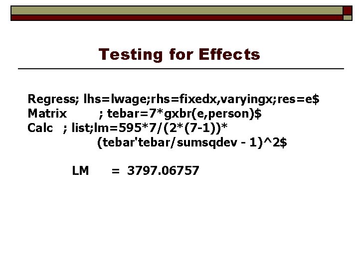
Testing for Effects: LM Test

Application: Cornwell-Rupert

Testing for Effects Regress; lhs=lwage; rhs=fixedx, varyingx; res=e$ Matrix ; tebar=7*gxbr(e, person)$ Calc ; list; lm=595*7/(2*(7 -1))* (tebar'tebar/sumsqdev - 1)^2$ LM = 3797. 06757

Hausman Test for FE vs. RE Estimator FGLS (Random Effects) Random Effects E[ci|Xi] = 0 Consistent and Efficient Fixed Effects E[ci|Xi] ≠ 0 Inconsistent LSDV (Fixed Effects) Consistent Inefficient Consistent Possibly Efficient

Hausman Test for Effects β does not contain the constant term in the preceding.

Computing the Hausman Statistic β does not contain the constant term in the preceding.

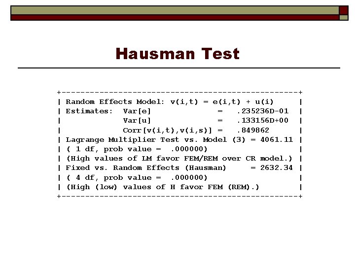
Hausman Test +-------------------------+ | Random Effects Model: v(i, t) = e(i, t) + u(i) | | Estimates: Var[e] =. 235236 D-01 | | Var[u] =. 133156 D+00 | | Corr[v(i, t), v(i, s)] =. 849862 | | Lagrange Multiplier Test vs. Model (3) = 4061. 11 | | ( 1 df, prob value =. 000000) | | (High values of LM favor FEM/REM over CR model. ) | | Fixed vs. Random Effects (Hausman) = 2632. 34 | | ( 4 df, prob value =. 000000) | | (High (low) values of H favor FEM (REM). ) | +-------------------------+

Wu (Variable Addition) Test Under the FE assumptions, the common effect is correlated with the group means. Add the group means to the RE model. If statistically significant, this suggests that the RE model is inappropriate.

Mundlak (Augmented) Regression +--------------+--------+--------+-----+ |Variable| Coefficient | Standard Error |b/St. Er. |P[|Z|>z]| Mean of X| +--------------+--------+--------+-----+ |EXPBAR | -. 08769***. 00162096 -54. 099. 0000 19. 853782| |OCCBAR | -. 14806***. 03623348 -4. 086. 0000. 5111645| |SMSABAR |. 21707***. 03209640 6. 763. 0000. 6537815| |MSBAR |. 14855***. 05087686 2. 920. 0035. 8144058| |UNYNBAR |. 07831**. 03257465 2. 404. 0162. 3639856| |WKSBAR |. 00857**. 00362039 2. 367. 0179 46. 811525| |INDBAR |. 03998. 02966215 1. 348. 1777. 3954382| |SOUTHBAR| -. 05487. 04293224 -1. 278. 2012. 2902761| |EXP |. 11448***. 00225862 50. 684. 0000 19. 853782| |EXPSQ | -. 00045***. 483957 D-04 -9. 304. 0000 514. 40504| |OCC | -. 02122. 01380348 -1. 537. 1243. 5111645| |SMSA | -. 04237**. 01945829 -2. 178. 0294. 6537815| |MS | -. 02969. 01901293 -1. 561. 1184. 8144058| |FEM | -. 31359***. 05419945 -5. 786. 0000. 1126050| |UNION |. 03268**. 01494574 2. 187. 0288. 3639856| |ED |. 05150***. 00550816 9. 349. 0000 12. 845378| |BLK | -. 15768***. 04463738 -3. 533. 0004. 0722689| |WKS |. 00081. 00060031 1. 354. 1759 46. 811525| |IND |. 01909. 01546993 1. 234. 2171. 3954382| |SOUTH | -. 00176. 03435229 -. 051. 9592. 2902761| |Constant| 5. 15038***. 20122987 25. 595. 0000 | +----------------------------------+

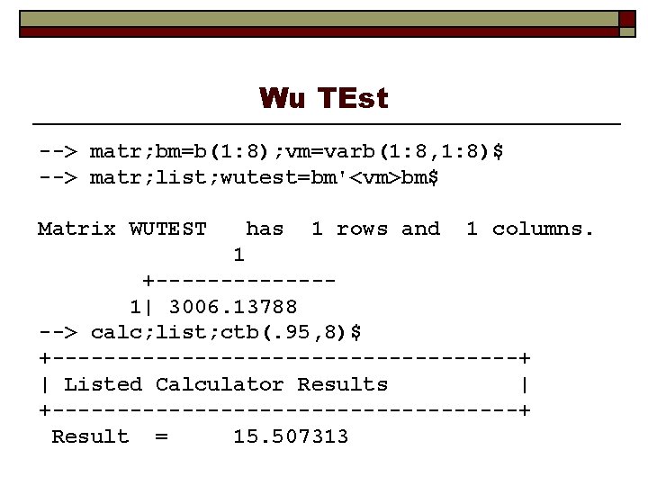
Wu TEst --> matr; bm=b(1: 8); vm=varb(1: 8, 1: 8)$ --> matr; list; wutest=bm'<vm>bm$ Matrix WUTEST has 1 rows and 1 columns. 1 +-------1| 3006. 13788 --> calc; list; ctb(. 95, 8)$ +------------------+ | Listed Calculator Results | +------------------+ Result = 15. 507313