Econometrics Chengyuan Yin School of Mathematics Econometrics 23

Econometrics Chengyuan Yin School of Mathematics

Econometrics 23. Discrete Choice Modeling

A Microeconomics Platform o o o Consumers Maximize Utility (!!!) Fundamental Choice Problem: Maximize U(x 1, x 2, …) subject to prices and budget constraints A Crucial Result for the Classical Problem: n n o Indirect Utility Function: V = V(p, I) Demand System of Continuous Choices The Integrability Problem: Utility is not revealed by demands

Theory for Discrete Choice o o Theory is silent about discrete choices Translation to discrete choice n n n o o o Choice sets and consideration sets – consumers simplify choice situations Implication for choice among a set of discrete alternatives Commonalities and uniqueness n n n o Existence of well defined utility indexes: Completeness of rankings Rationality: Utility maximization Axioms of revealed preferences Does this allow us to build “models? ” What common elements can be assumed? How can we account for heterogeneity? Revealed choices do not reveal utility, only rankings which are scale invariant

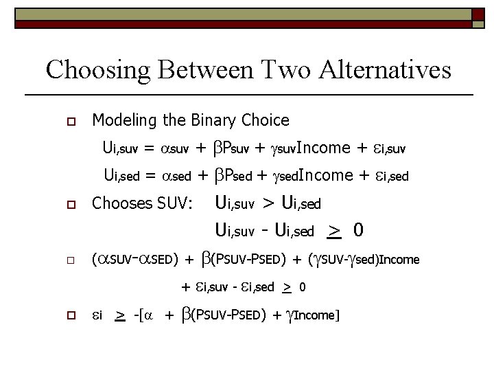
Choosing Between Two Alternatives o Modeling the Binary Choice Ui, suv = suv + Psuv + suv. Income + i, suv Ui, sed = sed + Psed + sed. Income + i, sed o o o Ui, suv > Ui, sed Ui, suv - Ui, sed > 0 ( SUV- SED) + (PSUV-PSED) + ( SUV- sed)Income + i, suv - i, sed > 0 i > -[ + (PSUV-PSED) + Income] Chooses SUV:

What Can Be Learned from the Data? (A Sample of Consumers, i = 1, …, N) • Are the attributes “relevant? ” • Predicting behavior - Individual - Aggregate • Analyze changes in behavior when attributes change

Application o o o 210 Commuters Between Sydney and Melbourne Available modes = Air, Train, Bus, Car Observed: n n n o Choice Attributes: Cost, terminal time, other Characteristics: Household income First application: Fly or Other

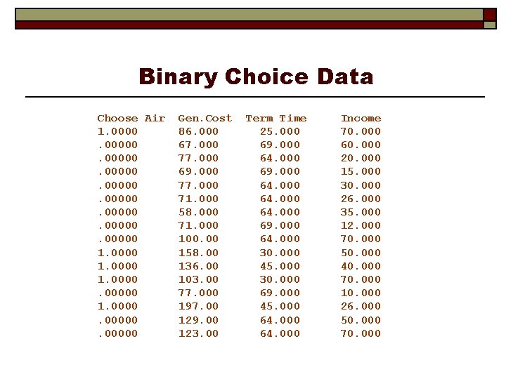
Binary Choice Data Choose Air 1. 00000 1. 00000 Gen. Cost 86. 000 67. 000 77. 000 69. 000 77. 000 71. 000 58. 000 71. 000 100. 00 158. 00 136. 00 103. 00 77. 000 197. 00 129. 00 123. 00 Term Time 25. 000 69. 000 64. 000 30. 000 45. 000 30. 000 69. 000 45. 000 64. 000 Income 70. 000 60. 000 20. 000 15. 000 30. 000 26. 000 35. 000 12. 000 70. 000 50. 000 40. 000 70. 000 10. 000 26. 000 50. 000 70. 000

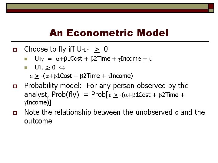
An Econometric Model o Choose to fly iff UFLY > 0 n n o Ufly = + 1 Cost + 2 Time + Income + Ufly > 0 > -( + 1 Cost + 2 Time + Income) Probability model: For any person observed by the analyst, Prob(fly) = Prob[ > -( + 1 Cost + 2 Time + Income)] o Note the relationship between the unobserved and the outcome

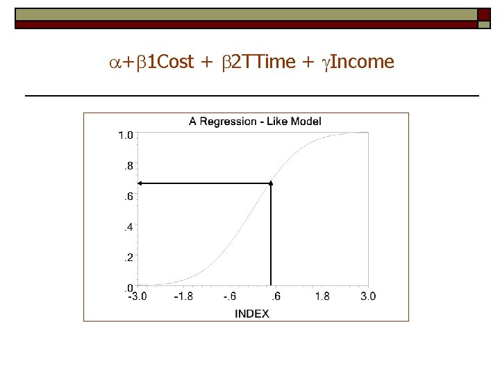
+ 1 Cost + 2 TTime + Income

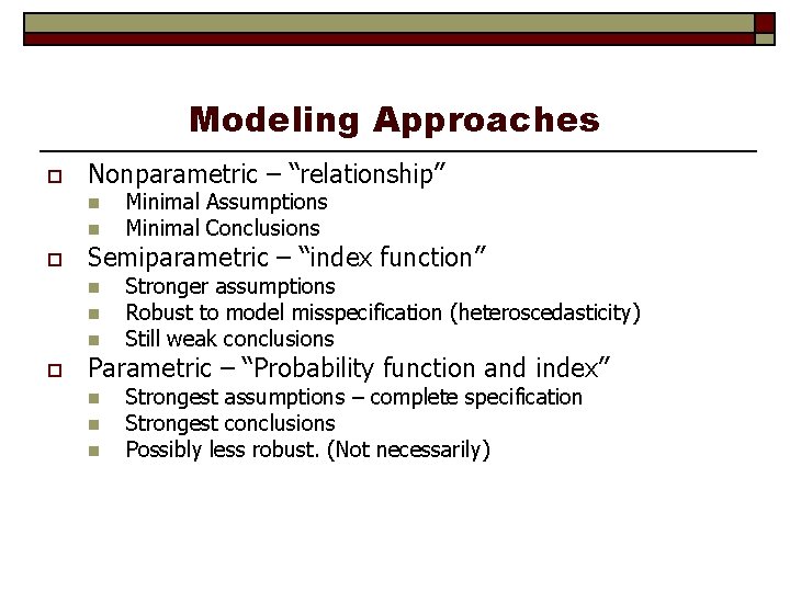
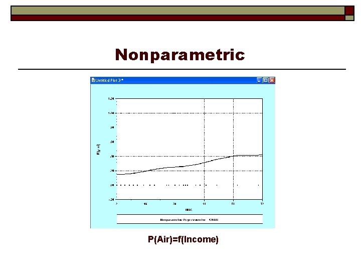
Modeling Approaches o Nonparametric – “relationship” n n o Semiparametric – “index function” n n n o Minimal Assumptions Minimal Conclusions Stronger assumptions Robust to model misspecification (heteroscedasticity) Still weak conclusions Parametric – “Probability function and index” n n n Strongest assumptions – complete specification Strongest conclusions Possibly less robust. (Not necessarily)

Nonparametric P(Air)=f(Income)

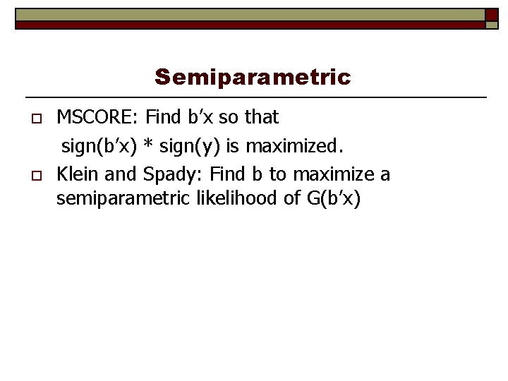
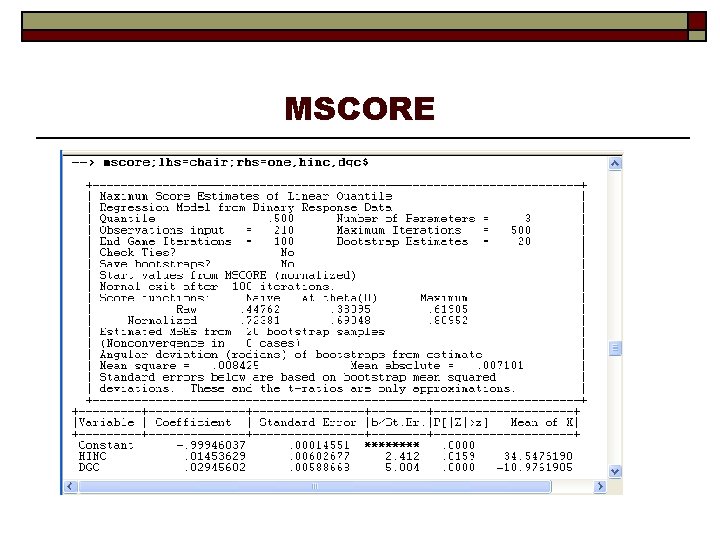
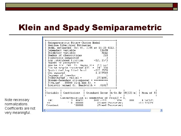
Semiparametric o o MSCORE: Find b’x so that sign(b’x) * sign(y) is maximized. Klein and Spady: Find b to maximize a semiparametric likelihood of G(b’x)

MSCORE

Klein and Spady Semiparametric Note necessary normalizations. Coefficients are not very meaningful.

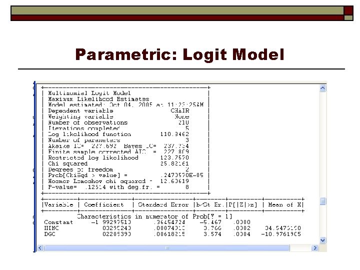
Parametric: Logit Model

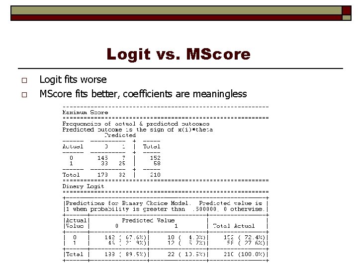
Logit vs. MScore o o Logit fits worse MScore fits better, coefficients are meaningless

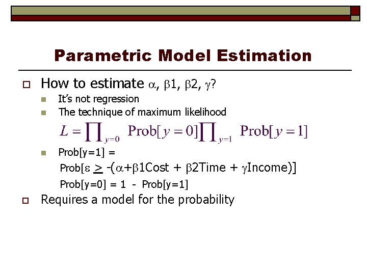
Parametric Model Estimation o How to estimate , 1, 2, ? n It’s not regression The technique of maximum likelihood n Prob[y=1] = n Prob[ > -( + 1 Cost + 2 Time + Income)] Prob[y=0] = 1 - Prob[y=1] o Requires a model for the probability

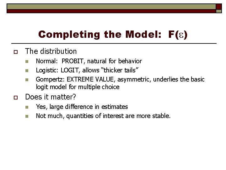
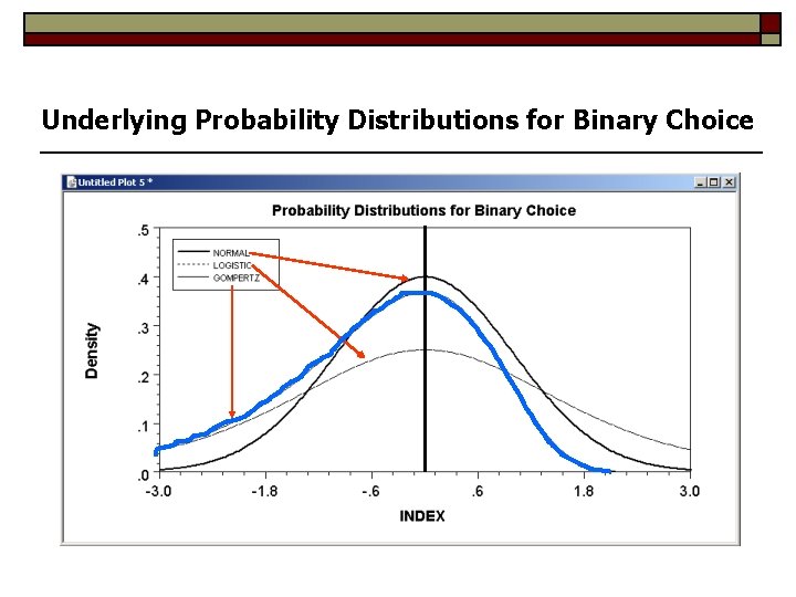
Completing the Model: F( ) o The distribution n o Normal: PROBIT, natural for behavior Logistic: LOGIT, allows “thicker tails” Gompertz: EXTREME VALUE, asymmetric, underlies the basic logit model for multiple choice Does it matter? n n Yes, large difference in estimates Not much, quantities of interest are more stable.

Underlying Probability Distributions for Binary Choice

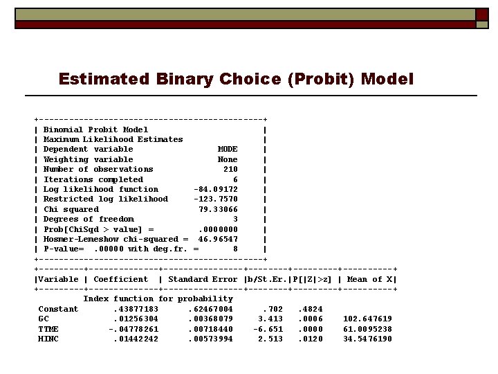
Estimated Binary Choice (Probit) Model +-----------------------+ | Binomial Probit Model | | Maximum Likelihood Estimates | | Dependent variable MODE | | Weighting variable None | | Number of observations 210 | | Iterations completed 6 | | Log likelihood function -84. 09172 | | Restricted log likelihood -123. 7570 | | Chi squared 79. 33066 | | Degrees of freedom 3 | | Prob[Chi. Sqd > value] =. 0000000 | | Hosmer-Lemeshow chi-squared = 46. 96547 | | P-value=. 00000 with deg. fr. = 8 | +-----------------------+ +--------------+--------+---------+-----+ |Variable | Coefficient | Standard Error |b/St. Er. |P[|Z|>z] | Mean of X| +--------------+--------+---------+-----+ Index function for probability Constant. 43877183. 62467004. 702. 4824 GC. 01256304. 00368079 3. 413. 0006 102. 647619 TTME -. 04778261. 00718440 -6. 651. 0000 61. 0095238 HINC. 01442242. 00573994 2. 513. 0120 34. 5476190

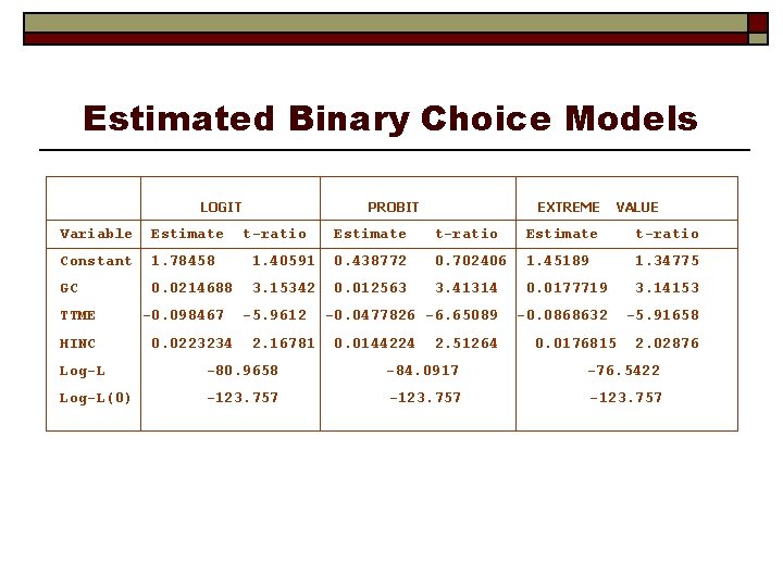
Estimated Binary Choice Models LOGIT Variable Estimate Constant 1. 78458 GC 0. 0214688 TTME HINC -0. 098467 0. 0223234 PROBIT t-ratio EXTREME VALUE Estimate t-ratio 1. 40591 0. 438772 0. 702406 1. 45189 1. 34775 3. 15342 0. 012563 3. 41314 0. 0177719 3. 14153 -0. 0477826 -6. 65089 -0. 0868632 -5. 91658 -5. 9612 2. 16781 0. 0144224 2. 51264 0. 0176815 2. 02876 Log-L -80. 9658 -84. 0917 -76. 5422 Log-L(0) -123. 757

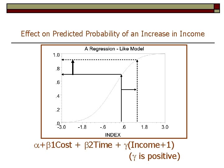
Effect on Predicted Probability of an Increase in Income + 1 Cost + 2 Time + (Income+1) ( is positive)

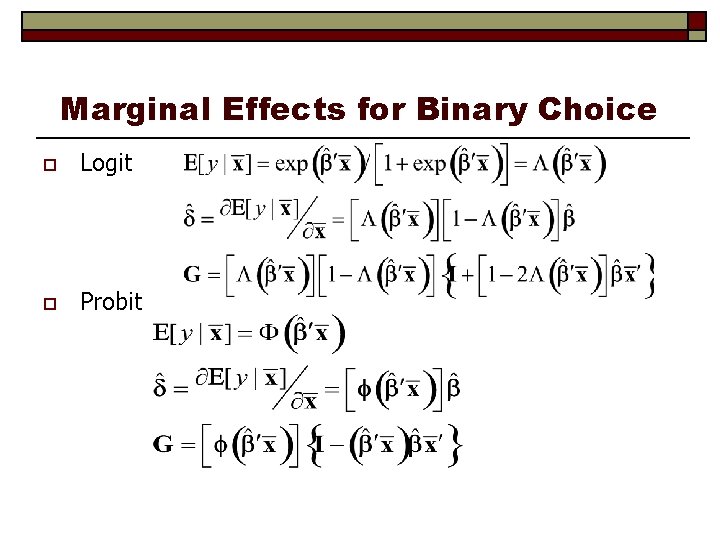
Marginal Effects in Probability Models Prob[Outcome] = some F( + 1 Cost…) o “Partial effect” = F( + 1 Cost…) / ”x” (derivative) o n n Partial effects are derivatives Result varies with model o o n Logit: F( + 1 Cost…) / x = Prob * (1 -Prob) * Probit: F( + 1 Cost…) / x = Normal density Scaling usually erases model differences

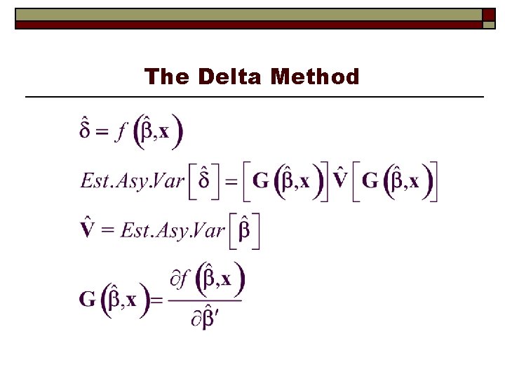
The Delta Method

Marginal Effects for Binary Choice o Logit o Probit

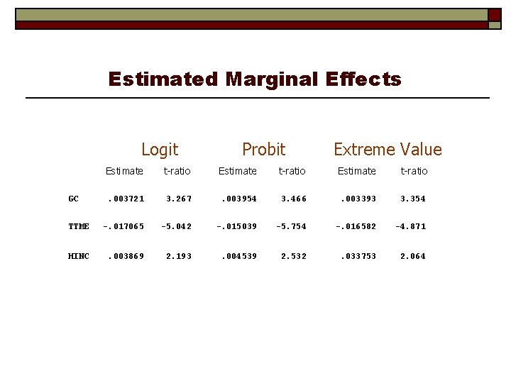
Estimated Marginal Effects Logit Probit Extreme Value Estimate t-ratio . 003721 3. 267 . 003954 3. 466 . 003393 3. 354 TTME -. 017065 -5. 042 -. 015039 -5. 754 -. 016582 -4. 871 HINC . 003869 2. 193 . 004539 2. 532 . 033753 2. 064 GC

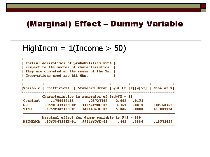
Marginal Effect for a Dummy Variable o o o Prob[yi = 1|xi, di] = F( ’xi+ di) =conditional mean Marginal effect of d Prob[yi = 1|xi, di=1]=Prob[yi= 1|xi, di=0] Logit:

(Marginal) Effect – Dummy Variable High. Incm = 1(Income > 50) +----------------------+ | Partial derivatives of probabilities with | | respect to the vector of characteristics. | | They are computed at the means of the Xs. | | Observations used are All Obs. | +----------------------+ +--------------+--------+---------+-----+ |Variable | Coefficient | Standard Error |b/St. Er. |P[|Z|>z] | Mean of X| +--------------+--------+---------+-----+ Characteristics in numerator of Prob[Y = 1] Constant. 4750039483. 23727762 2. 002. 0453 GC. 3598131572 E-02. 11354298 E-02 3. 169. 0015 102. 64762 TTME -. 1759234212 E-01. 34866343 E-02 -5. 046. 0000 61. 009524 Marginal effect for dummy variable is P|1 - P|0. HIGHINCM. 8565367181 E-01. 99346656 E-01. 862. 3886 . 18571429

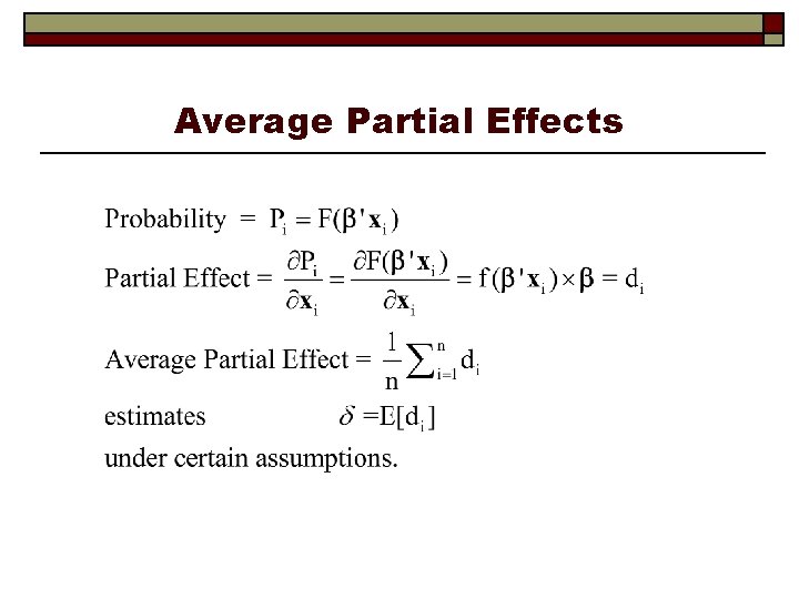
Computing Effects o Compute at the data means? n n o Simple Inference is well defined Average the individual effects n n n More appropriate? Asymptotic standard errors. (Not done correctly in the literature – terms are correlated!) Is testing about marginal effects meaningful?

Average Partial Effects

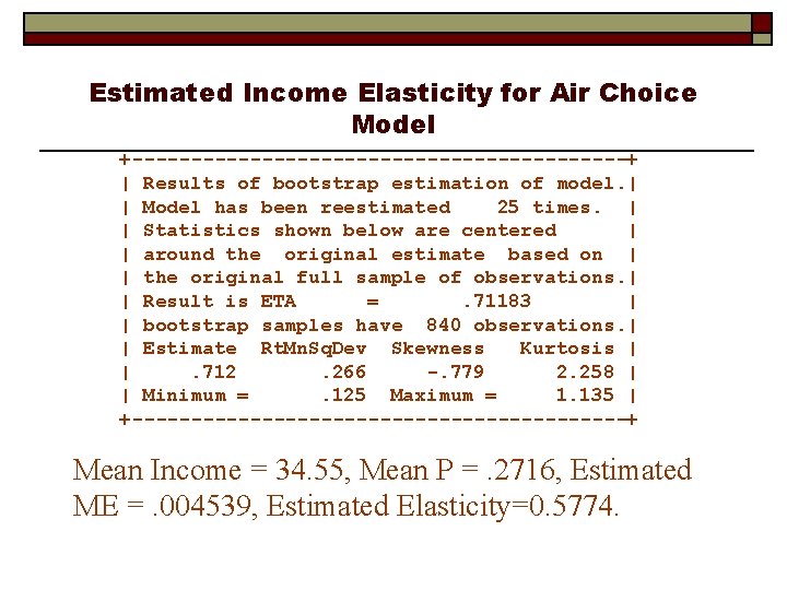
Elasticities o Elasticity = o How to compute standard errors? n n Delta method Bootstrap o o Bootstrap the individual elasticities? (Will neglect variation in parameter estimates. ) Bootstrap model estimation?

Estimated Income Elasticity for Air Choice Model +---------------------+ | Results of bootstrap estimation of model. | | Model has been reestimated 25 times. | | Statistics shown below are centered | | around the original estimate based on | | the original full sample of observations. | | Result is ETA =. 71183 | | bootstrap samples have 840 observations. | | Estimate Rt. Mn. Sq. Dev Skewness Kurtosis | |. 712. 266 -. 779 2. 258 | | Minimum =. 125 Maximum = 1. 135 | +---------------------+ Mean Income = 34. 55, Mean P =. 2716, Estimated ME =. 004539, Estimated Elasticity=0. 5774.

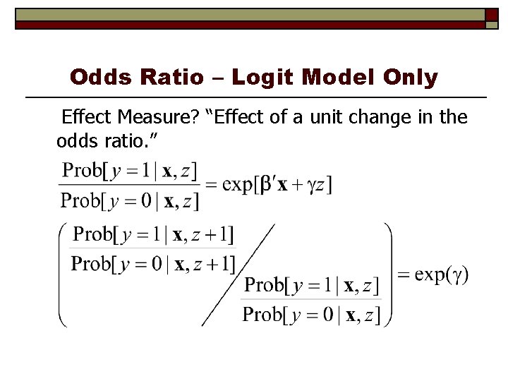
Odds Ratio – Logit Model Only Effect Measure? “Effect of a unit change in the odds ratio. ”

Ordered Outcomes o o o E. g. : Taste test, credit rating, course grade Underlying random preferences: Mapping to observed choices Strength of preferences Censoring and discrete measurement The nature of ordered data

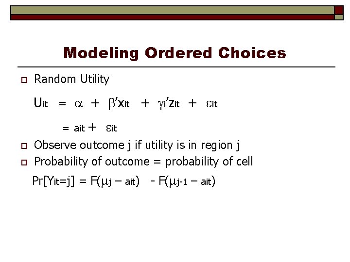
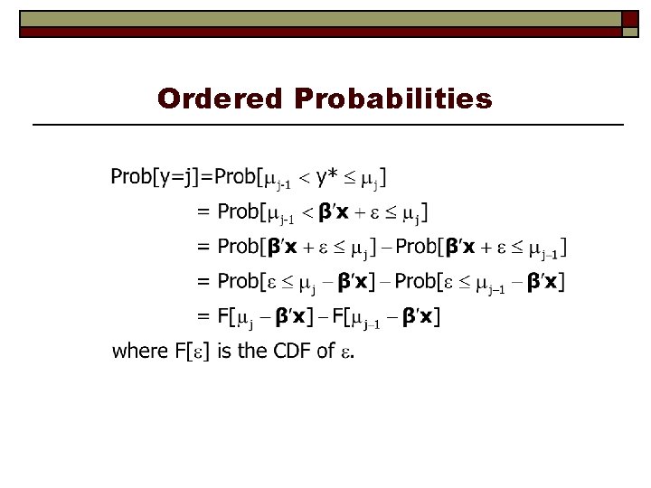
Modeling Ordered Choices o Random Utility Uit = + ’xit + i’zit + it = ait + o o it Observe outcome j if utility is in region j Probability of outcome = probability of cell Pr[Yit=j] = F( j – ait) - F( j-1 – ait)

Health Care Satisfaction (HSAT) Self administered survey: Health Care Satisfaction? (0 – 10) Continuous Preference Scale

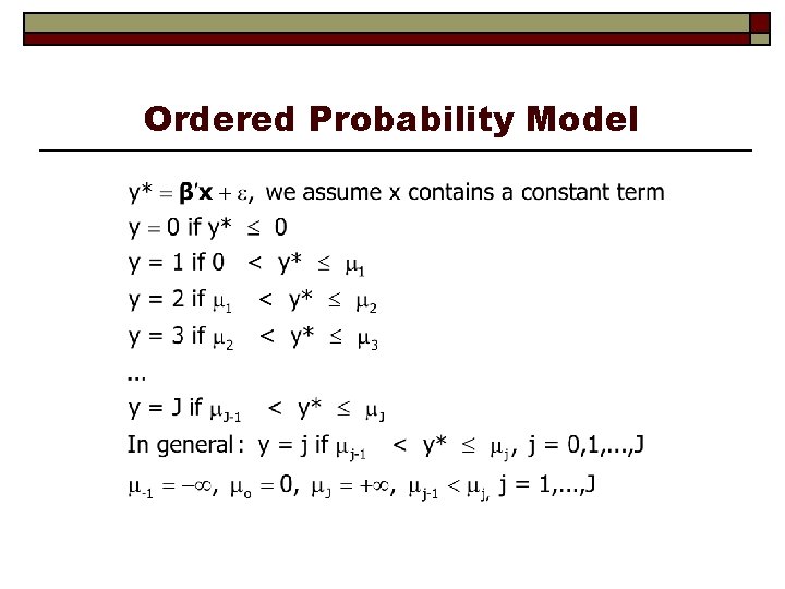
Ordered Probability Model

Ordered Probabilities

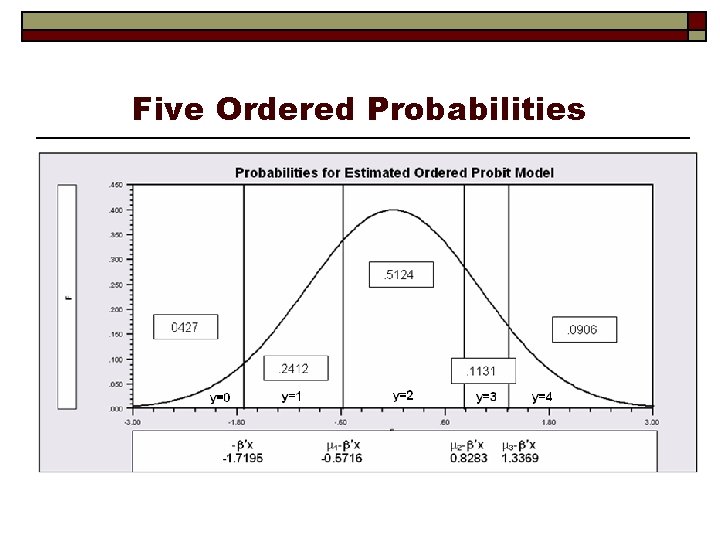
Five Ordered Probabilities

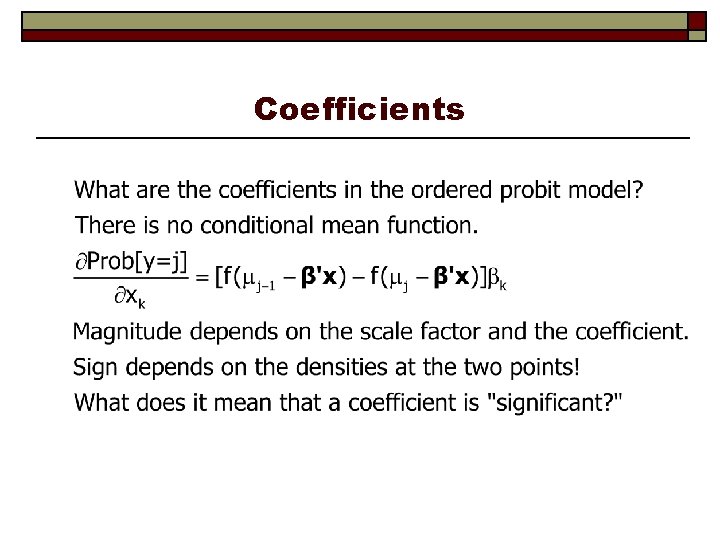
Coefficients

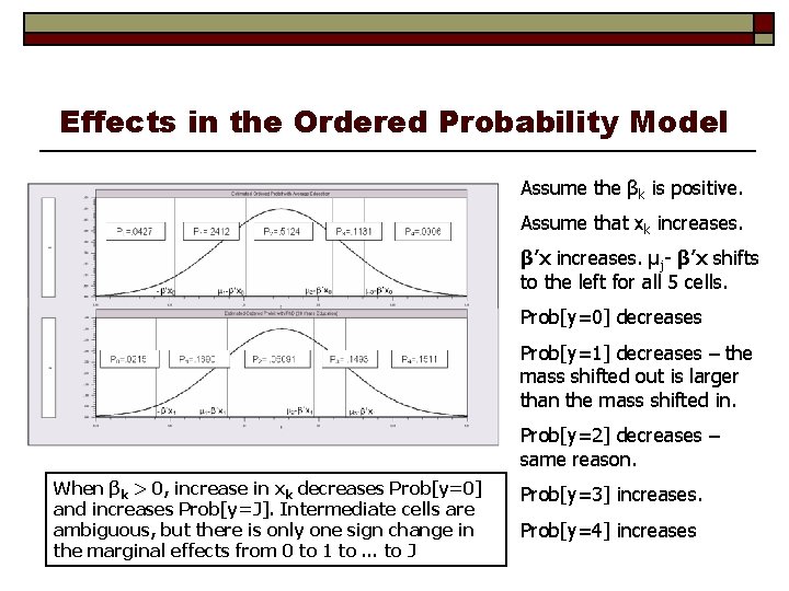
Effects in the Ordered Probability Model Assume the βk is positive. Assume that xk increases. β’x increases. μj- β’x shifts to the left for all 5 cells. Prob[y=0] decreases Prob[y=1] decreases – the mass shifted out is larger than the mass shifted in. Prob[y=2] decreases – same reason. When βk > 0, increase in xk decreases Prob[y=0] and increases Prob[y=J]. Intermediate cells are ambiguous, but there is only one sign change in the marginal effects from 0 to 1 to … to J Prob[y=3] increases. Prob[y=4] increases

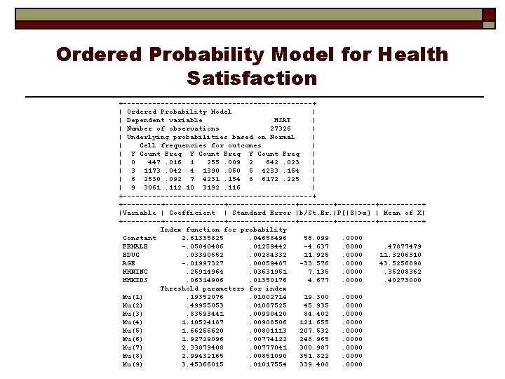
Ordered Probability Model for Health Satisfaction +-----------------------+ | Ordered Probability Model | | Dependent variable HSAT | | Number of observations 27326 | | Underlying probabilities based on Normal | | Cell frequencies for outcomes | | Y Count Freq | | 0 447. 016 1 255. 009 2 642. 023 | | 3 1173. 042 4 1390. 050 5 4233. 154 | | 6 2530. 092 7 4231. 154 8 6172. 225 | | 9 3061. 112 10 3192. 116 | +-----------------------+ +--------------+--------+---------+-----+ |Variable | Coefficient | Standard Error |b/St. Er. |P[|Z|>z] | Mean of X| +--------------+--------+---------+-----+ Index function for probability Constant 2. 61335825. 04658496 56. 099. 0000 FEMALE -. 05840486. 01259442 -4. 637. 0000. 47877479 EDUC. 03390552. 00284332 11. 925. 0000 11. 3206310 AGE -. 01997327. 00059487 -33. 576. 0000 43. 5256898 HHNINC. 25914964. 03631951 7. 135. 0000. 35208362 HHKIDS. 06314906. 01350176 4. 677. 0000. 40273000 Threshold parameters for index Mu(1). 19352076. 01002714 19. 300. 0000 Mu(2). 49955053. 01087525 45. 935. 0000 Mu(3). 83593441. 00990420 84. 402. 0000 Mu(4) 1. 10524187. 00908506 121. 655. 0000 Mu(5) 1. 66256620. 00801113 207. 532. 0000 Mu(6) 1. 92729096. 00774122 248. 965. 0000 Mu(7) 2. 33879408. 00777041 300. 987. 0000 Mu(8) 2. 99432165. 00851090 351. 822. 0000 Mu(9) 3. 45366015. 01017554 339. 408. 0000

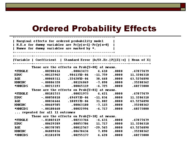
Ordered Probability Effects +--------------------------+ | Marginal effects for ordered probability model | | M. E. s for dummy variables are Pr[y|x=1]-Pr[y|x=0] | | Names for dummy variables are marked by *. | +--------------------------+ +--------------+--------+---------+-----+ |Variable | Coefficient | Standard Error |b/St. Er. |P[|Z|>z] | Mean of X| +--------------+--------+---------+-----+ These are the effects on Prob[Y=00] at means. *FEMALE. 00200414. 00043473 4. 610. 0000. 47877479 EDUC -. 00115962. 986135 D-04 -11. 759. 0000 11. 3206310 AGE. 00068311. 224205 D-04 30. 468. 0000 43. 5256898 HHNINC -. 00886328. 00124869 -7. 098. 0000. 35208362 *HHKIDS -. 00213193. 00045119 -4. 725. 0000. 40273000 These are the effects on Prob[Y=01] at means. *FEMALE. 00101533. 00021973 4. 621. 0000. 47877479 EDUC -. 00058810. 496973 D-04 -11. 834. 0000 11. 3206310 AGE. 00034644. 108937 D-04 31. 802. 0000 43. 5256898 HHNINC -. 00449505. 00063180 -7. 115. 0000. 35208362 *HHKIDS -. 00108460. 00022994 -4. 717. 0000. 40273000. . . repeated for all 11 outcomes These are the effects on Prob[Y=10] at means. *FEMALE -. 01082419. 00233746 -4. 631. 0000. 47877479 EDUC. 00629289. 00053706 11. 717. 0000 11. 3206310 AGE -. 00370705. 00012547 -29. 545. 0000 43. 5256898 HHNINC. 04809836. 00678434 7. 090. 0000. 35208362 *HHKIDS. 01181070. 00255177 4. 628. 0000. 40273000

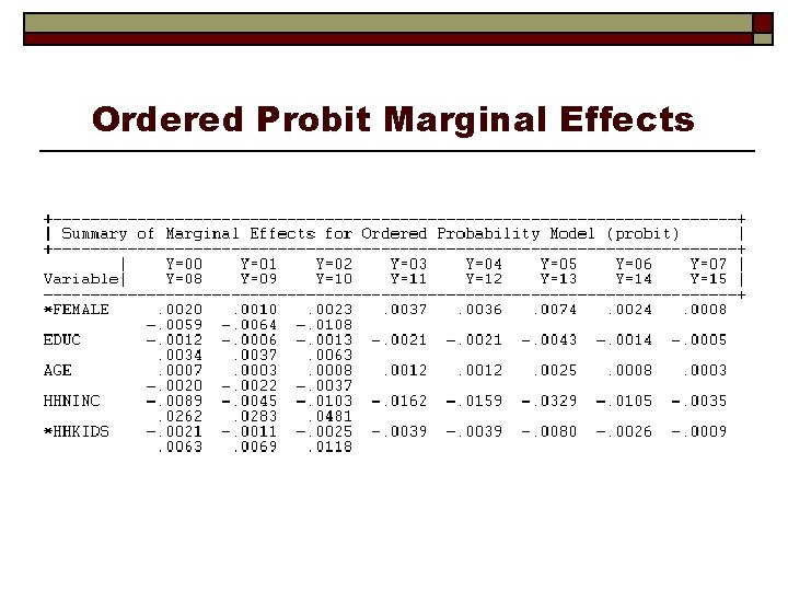
Ordered Probit Marginal Effects

Multinomial Choice Among J Alternatives • Random Utility Basis Uitj = ij + i ’xitj + i’zit + ijt i = 1, …, N; j = 1, …, J(i); t = 1, …, T(i) • Maximum Utility Assumption Individual i will Choose alternative j in choice setting t iff Uitk for all k j. • Underlying assumptions n n Smoothness of utilities Axioms: Transitive, Complete, Monotonic Uitj >

Utility Functions o o The linearity assumption and curvature The choice set Deterministic and random components: The “model” Generic vs. alternative specific components n n Attributes and characteristics Coefficients o o o Part worths Alternative specific constants Scaling

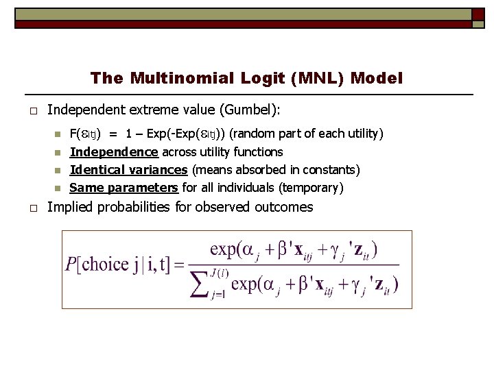
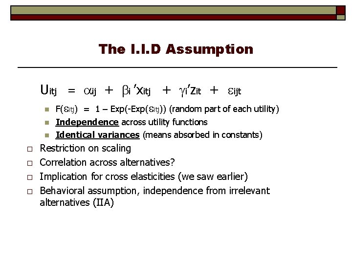
The Multinomial Logit (MNL) Model o Independent extreme value (Gumbel): n n o F( itj) = 1 – Exp(-Exp( itj)) (random part of each utility) Independence across utility functions Identical variances (means absorbed in constants) Same parameters for all individuals (temporary) Implied probabilities for observed outcomes

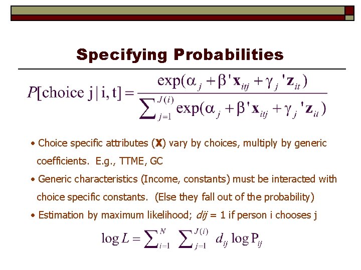
Specifying Probabilities • Choice specific attributes (X) vary by choices, multiply by generic coefficients. E. g. , TTME, GC • Generic characteristics (Income, constants) must be interacted with choice specific constants. (Else they fall out of the probability) • Estimation by maximum likelihood; dij = 1 if person i chooses j

Observed Data o Types of Data n n o o Individual choice Market shares Frequencies Ranks Attributes and Characteristics Choice Settings n n Cross section Repeated measurement (panel data)

Data on Discrete Choices Line 1 2 3 4 5 6 7 8 321 322 323 324 325 326 327 328 MODE AIR TRAIN BUS CAR TRAVEL. 00000 1. 0000 INVC 59. 000 31. 000 25. 000 10. 000 58. 000 31. 000 25. 000 11. 000 127. 00 109. 00 52. 000 50. 000 44. 000 25. 000 20. 000 5. 0000 INVT 100. 00 372. 00 417. 00 180. 00 68. 000 354. 00 399. 00 255. 00 193. 00 888. 00 1025. 0 892. 00 100. 00 351. 00 361. 00 180. 00 TTME 69. 000 34. 000 35. 00000 64. 000 44. 000 53. 00000 69. 000 34. 000 60. 00000 64. 000 44. 000 53. 00000 GC 70. 000 71. 000 70. 000 30. 000 68. 000 84. 000 85. 000 50. 000 148. 00 205. 00 163. 00 147. 00 59. 000 78. 000 75. 000 32. 000 HINC 35. 000 30. 000 60. 000 70. 000

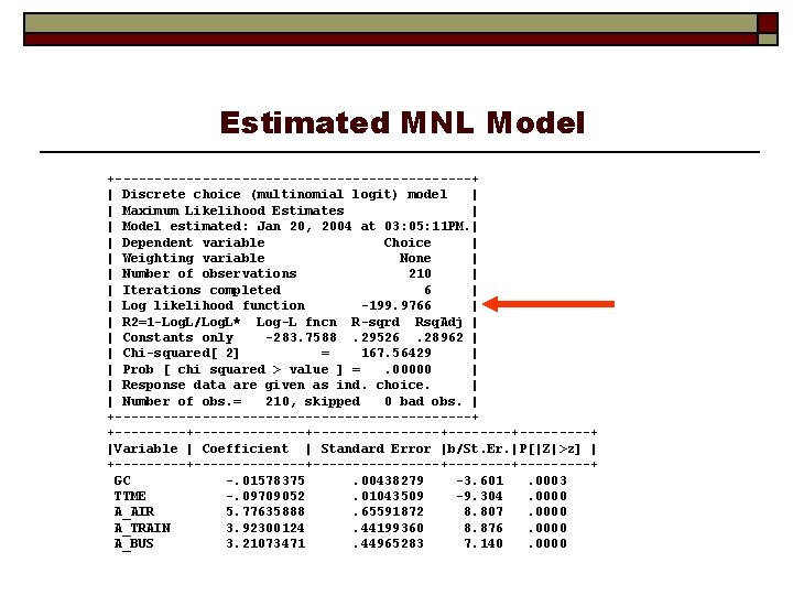
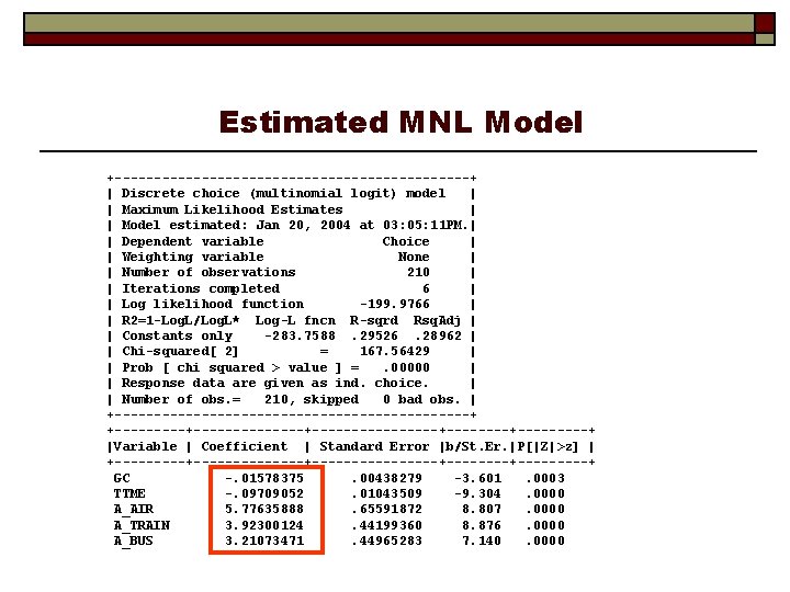
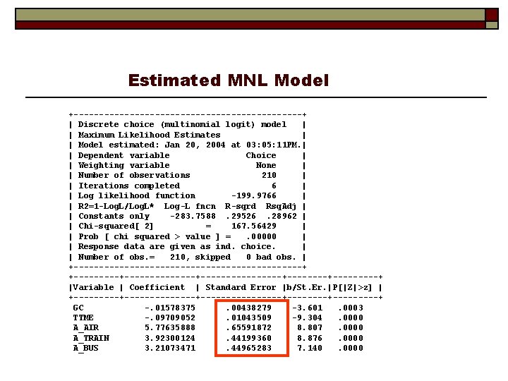
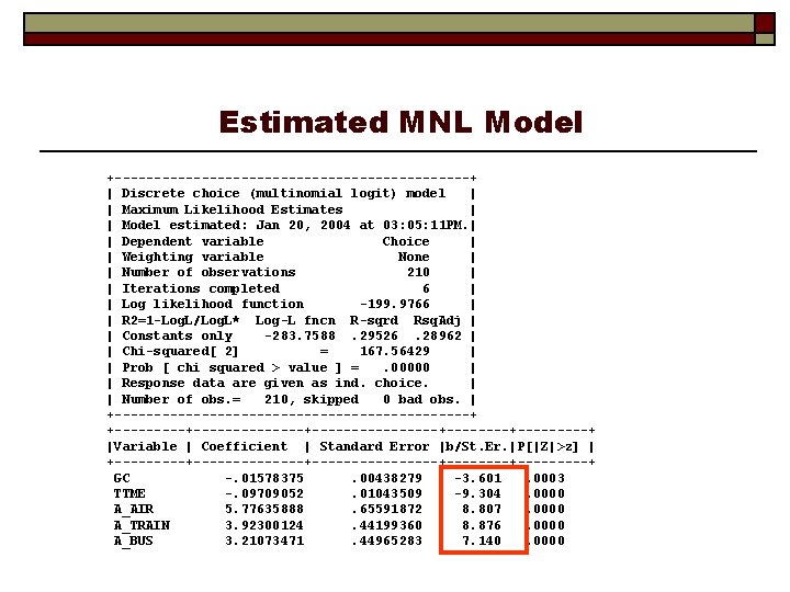
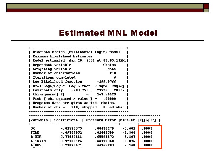
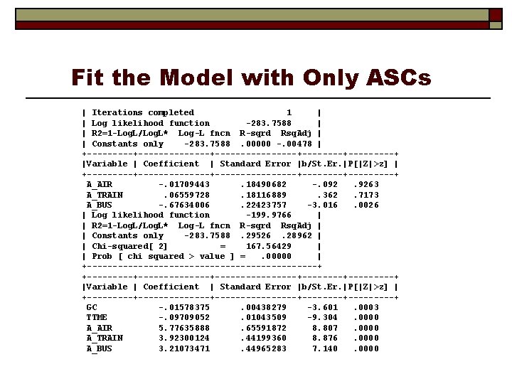
Estimated MNL Model +-----------------------+ | Discrete choice (multinomial logit) model | | Maximum Likelihood Estimates | | Model estimated: Jan 20, 2004 at 03: 05: 11 PM. | | Dependent variable Choice | | Weighting variable None | | Number of observations 210 | | Iterations completed 6 | | Log likelihood function -199. 9766 | | R 2=1 -Log. L/Log. L* Log-L fncn R-sqrd Rsq. Adj | | Constants only -283. 7588. 29526. 28962 | | Chi-squared[ 2] = 167. 56429 | | Prob [ chi squared > value ] =. 00000 | | Response data are given as ind. choice. | | Number of obs. = 210, skipped 0 bad obs. | +-----------------------+ +--------------+--------+---------+ |Variable | Coefficient | Standard Error |b/St. Er. |P[|Z|>z] | +--------------+--------+---------+ GC -. 01578375. 00438279 -3. 601. 0003 TTME -. 09709052. 01043509 -9. 304. 0000 A_AIR 5. 77635888. 65591872 8. 807. 0000 A_TRAIN 3. 92300124. 44199360 8. 876. 0000 A_BUS 3. 21073471. 44965283 7. 140. 0000

Estimated MNL Model +-----------------------+ | Discrete choice (multinomial logit) model | | Maximum Likelihood Estimates | | Model estimated: Jan 20, 2004 at 03: 05: 11 PM. | | Dependent variable Choice | | Weighting variable None | | Number of observations 210 | | Iterations completed 6 | | Log likelihood function -199. 9766 | | R 2=1 -Log. L/Log. L* Log-L fncn R-sqrd Rsq. Adj | | Constants only -283. 7588. 29526. 28962 | | Chi-squared[ 2] = 167. 56429 | | Prob [ chi squared > value ] =. 00000 | | Response data are given as ind. choice. | | Number of obs. = 210, skipped 0 bad obs. | +-----------------------+ +--------------+--------+---------+ |Variable | Coefficient | Standard Error |b/St. Er. |P[|Z|>z] | +--------------+--------+---------+ GC -. 01578375. 00438279 -3. 601. 0003 TTME -. 09709052. 01043509 -9. 304. 0000 A_AIR 5. 77635888. 65591872 8. 807. 0000 A_TRAIN 3. 92300124. 44199360 8. 876. 0000 A_BUS 3. 21073471. 44965283 7. 140. 0000

Estimated MNL Model +-----------------------+ | Discrete choice (multinomial logit) model | | Maximum Likelihood Estimates | | Model estimated: Jan 20, 2004 at 03: 05: 11 PM. | | Dependent variable Choice | | Weighting variable None | | Number of observations 210 | | Iterations completed 6 | | Log likelihood function -199. 9766 | | R 2=1 -Log. L/Log. L* Log-L fncn R-sqrd Rsq. Adj | | Constants only -283. 7588. 29526. 28962 | | Chi-squared[ 2] = 167. 56429 | | Prob [ chi squared > value ] =. 00000 | | Response data are given as ind. choice. | | Number of obs. = 210, skipped 0 bad obs. | +-----------------------+ +--------------+--------+---------+ |Variable | Coefficient | Standard Error |b/St. Er. |P[|Z|>z] | +--------------+--------+---------+ GC -. 01578375. 00438279 -3. 601. 0003 TTME -. 09709052. 01043509 -9. 304. 0000 A_AIR 5. 77635888. 65591872 8. 807. 0000 A_TRAIN 3. 92300124. 44199360 8. 876. 0000 A_BUS 3. 21073471. 44965283 7. 140. 0000

Estimated MNL Model +-----------------------+ | Discrete choice (multinomial logit) model | | Maximum Likelihood Estimates | | Model estimated: Jan 20, 2004 at 03: 05: 11 PM. | | Dependent variable Choice | | Weighting variable None | | Number of observations 210 | | Iterations completed 6 | | Log likelihood function -199. 9766 | | R 2=1 -Log. L/Log. L* Log-L fncn R-sqrd Rsq. Adj | | Constants only -283. 7588. 29526. 28962 | | Chi-squared[ 2] = 167. 56429 | | Prob [ chi squared > value ] =. 00000 | | Response data are given as ind. choice. | | Number of obs. = 210, skipped 0 bad obs. | +-----------------------+ +--------------+--------+---------+ |Variable | Coefficient | Standard Error |b/St. Er. |P[|Z|>z] | +--------------+--------+---------+ GC -. 01578375. 00438279 -3. 601. 0003 TTME -. 09709052. 01043509 -9. 304. 0000 A_AIR 5. 77635888. 65591872 8. 807. 0000 A_TRAIN 3. 92300124. 44199360 8. 876. 0000 A_BUS 3. 21073471. 44965283 7. 140. 0000

Estimated MNL Model +-----------------------+ | Discrete choice (multinomial logit) model | | Maximum Likelihood Estimates | | Model estimated: Jan 20, 2004 at 03: 05: 11 PM. | | Dependent variable Choice | | Weighting variable None | | Number of observations 210 | | Iterations completed 6 | | Log likelihood function -199. 9766 | | R 2=1 -Log. L/Log. L* Log-L fncn R-sqrd Rsq. Adj | | Constants only -283. 7588. 29526. 28962 | | Chi-squared[ 2] = 167. 56429 | | Prob [ chi squared > value ] =. 00000 | | Response data are given as ind. choice. | | Number of obs. = 210, skipped 0 bad obs. | +-----------------------+ +--------------+--------+---------+ |Variable | Coefficient | Standard Error |b/St. Er. |P[|Z|>z] | +--------------+--------+---------+ GC -. 01578375. 00438279 -3. 601. 0003 TTME -. 09709052. 01043509 -9. 304. 0000 A_AIR 5. 77635888. 65591872 8. 807. 0000 A_TRAIN 3. 92300124. 44199360 8. 876. 0000 A_BUS 3. 21073471. 44965283 7. 140. 0000

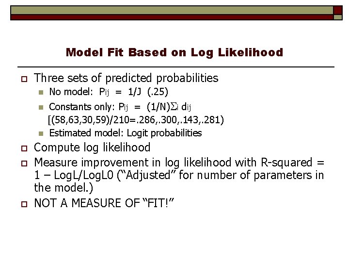
Model Fit Based on Log Likelihood o Three sets of predicted probabilities n n n o o o No model: Pij = 1/J (. 25) Constants only: Pij = (1/N) i dij [(58, 63, 30, 59)/210=. 286, . 300, . 143, . 281) Estimated model: Logit probabilities Compute log likelihood Measure improvement in log likelihood with R-squared = 1 – Log. L/Log. L 0 (“Adjusted” for number of parameters in the model. ) NOT A MEASURE OF “FIT!”

Fit the Model with Only ASCs | Iterations completed 1 | | Log likelihood function -283. 7588 | | R 2=1 -Log. L/Log. L* Log-L fncn R-sqrd Rsq. Adj | | Constants only -283. 7588. 00000 -. 00478 | +--------------+--------+---------+ |Variable | Coefficient | Standard Error |b/St. Er. |P[|Z|>z] | +--------------+--------+---------+ A_AIR -. 01709443. 18490682 -. 092. 9263 A_TRAIN. 06559728. 18116889. 362. 7173 A_BUS -. 67634006. 22423757 -3. 016. 0026 | Log likelihood function -199. 9766 | | R 2=1 -Log. L/Log. L* Log-L fncn R-sqrd Rsq. Adj | | Constants only -283. 7588. 29526. 28962 | | Chi-squared[ 2] = 167. 56429 | | Prob [ chi squared > value ] =. 00000 | +-----------------------+ +--------------+--------+---------+ |Variable | Coefficient | Standard Error |b/St. Er. |P[|Z|>z] | +--------------+--------+---------+ GC -. 01578375. 00438279 -3. 601. 0003 TTME -. 09709052. 01043509 -9. 304. 0000 A_AIR 5. 77635888. 65591872 8. 807. 0000 A_TRAIN 3. 92300124. 44199360 8. 876. 0000 A_BUS 3. 21073471. 44965283 7. 140. 0000

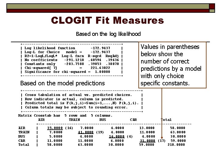
CLOGIT Fit Measures Based on the log likelihood +-----------------------+ | Log likelihood function -172. 9437 | | Log-L for Choice model = -172. 9437 | | R 2=1 -Log. L/Log. L* Log-L fncn R-sqrd Rsq. Adj | | No coefficients -291. 1218. 40594. 39636 | | Constants only -283. 7588. 39053. 38070 | | Chi-squared[ 7] = 221. 63022 | | Significance for chi-squared = 1. 00000 | +-----------------------+ Based on the model predictions Values in parentheses below show the number of correct predictions by a model with only choice specific constants. +---------------------------+ | Cross tabulation of actual vs. predicted choices. | | Row indicator is actual, column is predicted. | | Predicted total is F(k, j, i)=Sum(i=1, . . . , N) P(k, j, i). | | Column totals may be subject to rounding error. | +---------------------------+ Matrix Crosstab has 5 rows and 5 columns. AIR TRAIN BUS CAR Total +-----------------------------------AIR | 35. 0000 (16) 7. 0000 4. 0000 13. 0000 58. 0000 TRAIN | 7. 0000 41. 0000 (19) 4. 0000 11. 0000 63. 0000 BUS | 5. 0000 4. 0000 16. 0000 (4) 4. 0000 30. 0000 CAR | 11. 0000 6. 0000 31. 0000 (17) 59. 0000 Total | 58. 0000 63. 0000 30. 0000 59. 0000 210. 0000

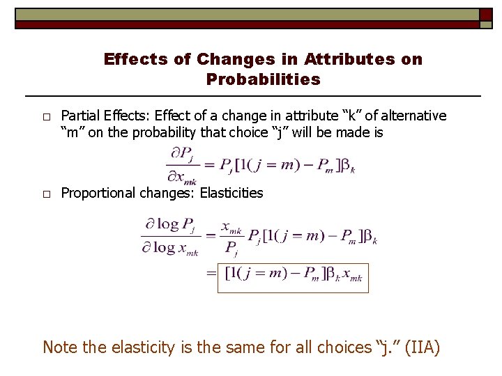
Effects of Changes in Attributes on Probabilities o Partial Effects: Effect of a change in attribute “k” of alternative “m” on the probability that choice “j” will be made is o Proportional changes: Elasticities Note the elasticity is the same for all choices “j. ” (IIA)

Elasticities for CLOGIT o o Request: ; Effects: attribute (choices where changes occur ) ; Effects: INVT(*) (INVT changes in all choices) +---------------------------------+ | Elasticity Averaged over observations. | | Effects on probabilities of all choices in the model: | | * indicates direct Elasticity effect of the attribute. | | Trunk Limb Branch Choice Effect| | Attribute is INVT in choice AIR | | * Choice=AIR. 000 -1. 336 | | Choice=TRAIN. 000. 535 | | Choice=BUS. 000. 535 | | Choice=CAR. 000. 535 | | Attribute is INVT in choice TRAIN | | Choice=AIR. 000 2. 215 | | * Choice=TRAIN. 000 -6. 298 | | Choice=BUS. 000 2. 215 | | Choice=CAR. 000 2. 215 | | Attribute is INVT in choice BUS | | Choice=AIR. 000 1. 194 | | Choice=TRAIN. 000 1. 194 | | * Choice=BUS. 000 -7. 615 | | Choice=CAR. 000 1. 194 | | Attribute is INVT in choice CAR | | Choice=AIR. 000 2. 085 | | Choice=TRAIN. 000 2. 085 | | Choice=BUS. 000 2. 085 | | * Choice=CAR. 000 -5. 937 | +---------------------------------+ Own effect Cross effects Note the effect of IIA on the cross effects.

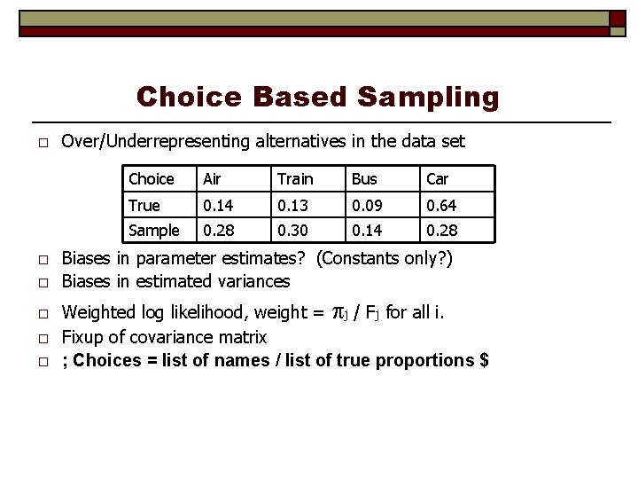
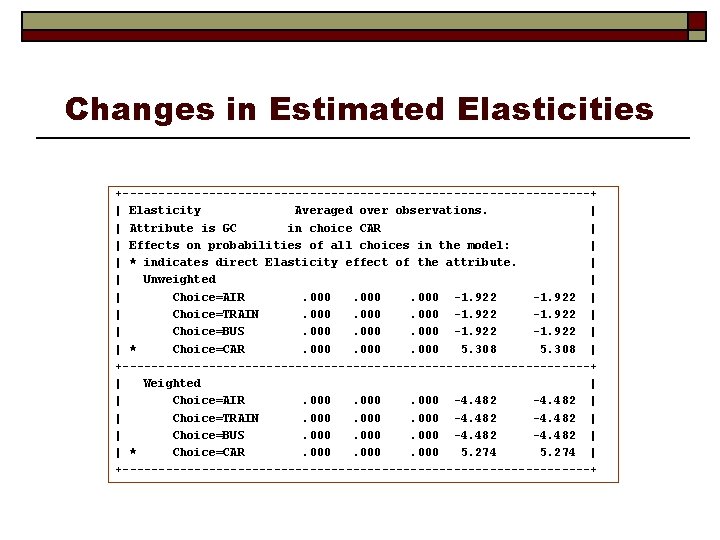
Choice Based Sampling o o o Over/Underrepresenting alternatives in the data set Choice Air Train Bus Car True 0. 14 0. 13 0. 09 0. 64 Sample 0. 28 0. 30 0. 14 0. 28 Biases in parameter estimates? (Constants only? ) Biases in estimated variances Weighted log likelihood, weight = j / Fj for all i. Fixup of covariance matrix ; Choices = list of names / list of true proportions $

Choice Based Sampling Estimators +--------------+--------+---------+ |Variable | Coefficient | Standard Error |b/St. Er. |P[|Z|>z] | +--------------+--------+---------+ Unweighted GC. 7577656131 E-01. 18331991 E-01 4. 134. 0000 TTME -. 1028868983. 11087157 E-01 -9. 280. 0000 INVT -. 1399485532 E-01. 26709164 E-02 -5. 240. 0000 INVC -. 8043945139 E-01. 19950713 E-01 -4. 032. 0001 A_AIR 4. 370346415 1. 0573353 4. 133. 0000 AIRx. HIN 1. 4275438233 E-02. 13061691 E-01. 327. 7434 A_TRAIN 5. 914073895. 68992964 8. 572. 0000 TRAx. HIN 2 -. 5907284040 E-01. 14709175 E-01 -4. 016. 0001 A_BUS 4. 462691316. 72332545 6. 170. 0000 BUSx. HIN 3 -. 2295037775 E-01. 15917353 E-01 -1. 442. 1493 +--------------+--------+---------+ Weighted GC. 1022492766. 22662522 E-01 4. 512. 0000 TTME -. 1361098346. 19321208 E-01 -7. 045. 0000 INVT -. 1772099171 E-01. 33128059 E-02 -5. 349. 0000 INVC -. 1035114747. 23306867 E-01 -4. 441. 0000 A_AIR 4. 525045167 1. 2865721 3. 517. 0004 AIRx. HIN 1. 7458987986 E-02. 13402559 E-01. 557. 5778 A_TRAIN 5. 532288683. 71701137 7. 716. 0000 TRAx. HIN 2 -. 6026155867 E-01. 17377917 E-01 -3. 468. 0005 A_BUS 4. 365784894. 78651423 5. 551. 0000 BUSx. HIN 3 -. 1956868658 E-01. 17288002 E-01 -1. 132. 2577

Changes in Estimated Elasticities +---------------------------------+ | Elasticity Averaged over observations. | | Attribute is GC in choice CAR | | Effects on probabilities of all choices in the model: | | * indicates direct Elasticity effect of the attribute. | | Unweighted | | Choice=AIR. 000 -1. 922 | | Choice=TRAIN. 000 -1. 922 | | Choice=BUS. 000 -1. 922 | | * Choice=CAR. 000 5. 308 | +---------------------------------+ | Weighted | | Choice=AIR. 000 -4. 482 | | Choice=TRAIN. 000 -4. 482 | | Choice=BUS. 000 -4. 482 | | * Choice=CAR. 000 5. 274 | +---------------------------------+

The I. I. D Assumption Uitj = ij + i ’xitj + i’zit + ijt n n n o o F( itj) = 1 – Exp(-Exp( itj)) (random part of each utility) Independence across utility functions Identical variances (means absorbed in constants) Restriction on scaling Correlation across alternatives? Implication for cross elasticities (we saw earlier) Behavioral assumption, independence from irrelevant alternatives (IIA)