Econometrics Chengyuan Yin School of Mathematics Econometrics 26



- Slides: 26

Econometrics Chengyuan Yin School of Mathematics

Econometrics 26. Time Series Data

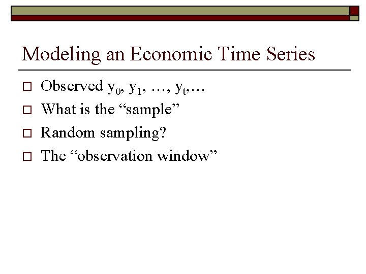
Modeling an Economic Time Series o o Observed y 0, y 1, …, yt, … What is the “sample” Random sampling? The “observation window”

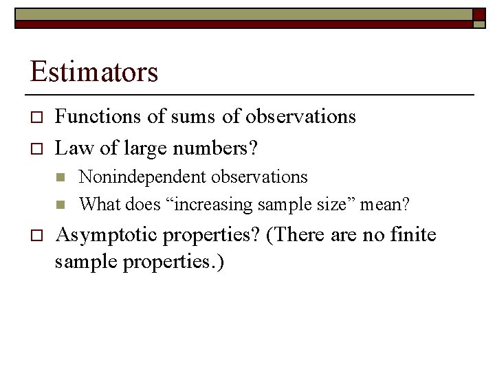
Estimators o o Functions of sums of observations Law of large numbers? n n o Nonindependent observations What does “increasing sample size” mean? Asymptotic properties? (There are no finite sample properties. )

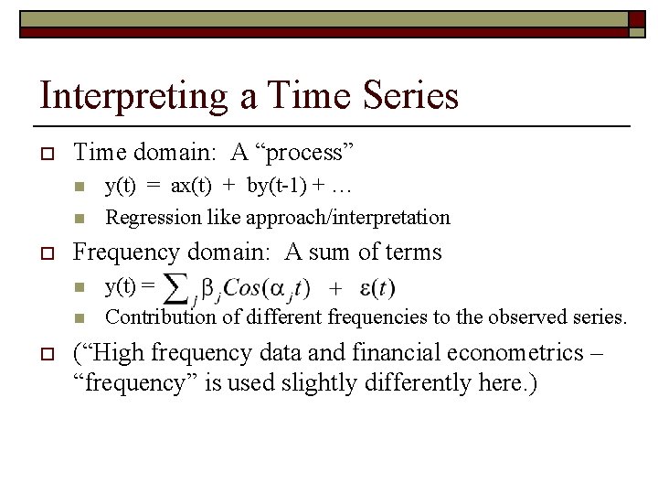
Interpreting a Time Series o Time domain: A “process” n n o Frequency domain: A sum of terms n n o y(t) = ax(t) + by(t-1) + … Regression like approach/interpretation y(t) = Contribution of different frequencies to the observed series. (“High frequency data and financial econometrics – “frequency” is used slightly differently here. )

For example, …

In parts…

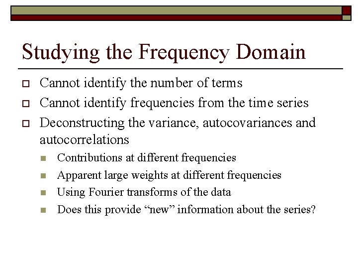
Studying the Frequency Domain o o o Cannot identify the number of terms Cannot identify frequencies from the time series Deconstructing the variance, autocovariances and autocorrelations n n Contributions at different frequencies Apparent large weights at different frequencies Using Fourier transforms of the data Does this provide “new” information about the series?

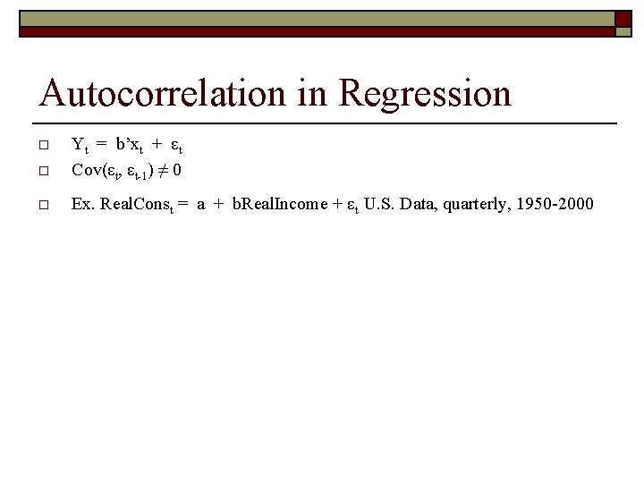
Autocorrelation in Regression o Yt = b’xt + εt Cov(εt, εt-1) ≠ 0 o Ex. Real. Const = a + b. Real. Income + εt U. S. Data, quarterly, 1950 -2000 o

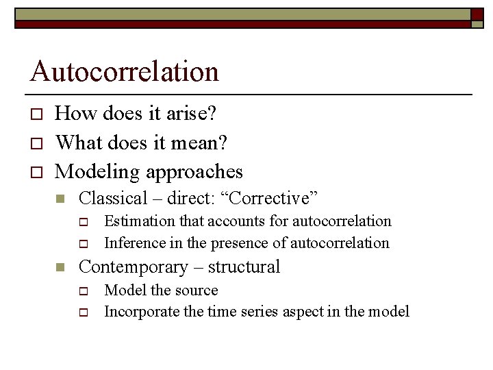
Autocorrelation o o o How does it arise? What does it mean? Modeling approaches n Classical – direct: “Corrective” o o n Estimation that accounts for autocorrelation Inference in the presence of autocorrelation Contemporary – structural o o Model the source Incorporate the time series aspect in the model

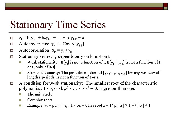
Stationary Time Series o o zt = b 1 yt-1 + b 2 yt-2 + … + b. Pyt-P + et Autocovariance: γk = Cov[yt, yt-k] Autocorrelation: k = γk / γ 0 Stationary series: γk depends only on k, not on t n n o Weak stationarity: E[yt] is not a function of t, E[yt * yt-s] is not a function of t or s, only of |t-s| Strong stationarity: The joint distribution of [yt, yt-1, …, yt-s] for any window of length s periods, is not a function of t or s. A condition for weak stationarity: The smallest root of the characteristic polynomial: 1 - b 1 z 1 - b 2 z 2 - … - b. Pz. P = 0, is greater than one. n n n The unit circle Complex roots Example: yt = yt-1 + ee, 1 - z = 0 has root z = 1/ , | z | > 1 => | | < 1.

Stationary vs. Nonstationary Series

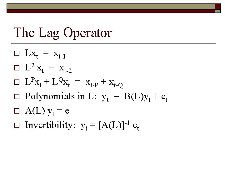
The Lag Operator o o o Lxt = xt-1 L 2 xt = xt-2 LPxt + LQxt = xt-P + xt-Q Polynomials in L: yt = B(L)yt + et A(L) yt = et Invertibility: yt = [A(L)]-1 et

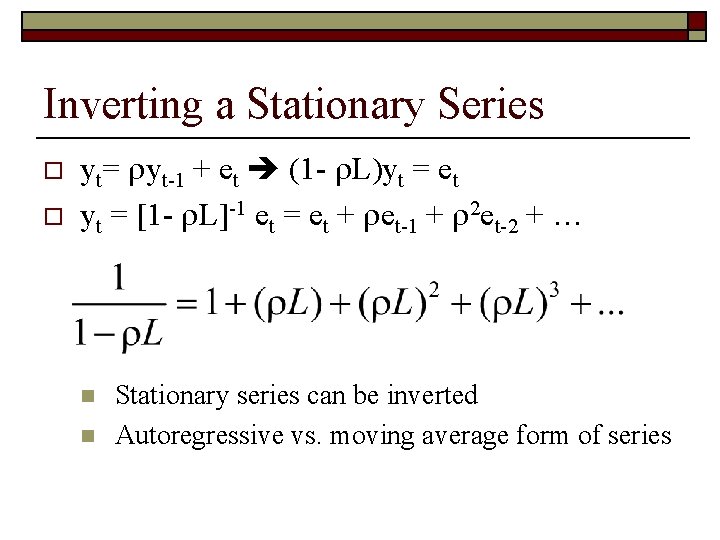
Inverting a Stationary Series o o yt= yt-1 + et (1 - L)yt = et yt = [1 - L]-1 et = et + et-1 + 2 et-2 + … n n Stationary series can be inverted Autoregressive vs. moving average form of series

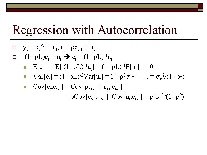
Regression with Autocorrelation o o yt = xt’b + et, et = et-1 + ut (1 - L)et = ut et = (1 - L)-1 ut n E[et] = E[ (1 - L)-1 ut] = (1 - L)-1 E[ut] = 0 n Var[et] = (1 - L)-2 Var[ut] = 1+ 2 u 2 + … = u 2/(1 - 2) n Cov[et, et-1] = Cov[ et-1 + ut, et-1] = = Cov[et-1, et-1]+Cov[ut, et-1] = u 2/(1 - 2)

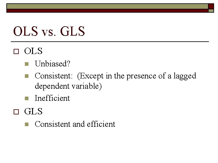
OLS vs. GLS o OLS n n n o Unbiased? Consistent: (Except in the presence of a lagged dependent variable) Inefficient GLS n Consistent and efficient

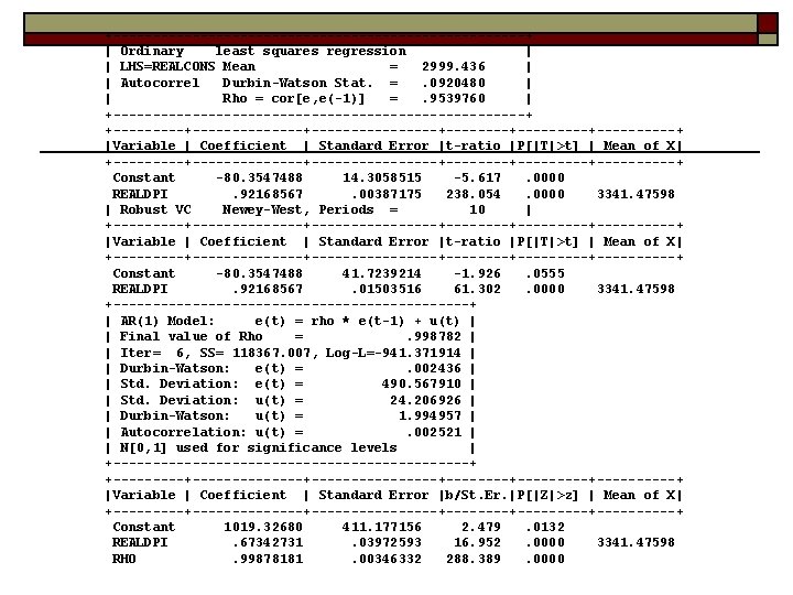
+--------------------------+ | Ordinary least squares regression | | LHS=REALCONS Mean = 2999. 436 | | Autocorrel Durbin-Watson Stat. =. 0920480 | | Rho = cor[e, e(-1)] =. 9539760 | +--------------------------+ +--------------+--------+---------+-----+ |Variable | Coefficient | Standard Error |t-ratio |P[|T|>t] | Mean of X| +--------------+--------+---------+-----+ Constant -80. 3547488 14. 3058515 -5. 617. 0000 REALDPI. 92168567. 00387175 238. 054. 0000 3341. 47598 | Robust VC Newey-West, Periods = 10 | +--------------+--------+---------+-----+ |Variable | Coefficient | Standard Error |t-ratio |P[|T|>t] | Mean of X| +--------------+--------+---------+-----+ Constant -80. 3547488 41. 7239214 -1. 926. 0555 REALDPI. 92168567. 01503516 61. 302. 0000 3341. 47598 +-----------------------+ | AR(1) Model: e(t) = rho * e(t-1) + u(t) | | Final value of Rho =. 998782 | | Iter= 6, SS= 118367. 007, Log-L=-941. 371914 | | Durbin-Watson: e(t) =. 002436 | | Std. Deviation: e(t) = 490. 567910 | | Std. Deviation: u(t) = 24. 206926 | | Durbin-Watson: u(t) = 1. 994957 | | Autocorrelation: u(t) =. 002521 | | N[0, 1] used for significance levels | +-----------------------+ +--------------+--------+---------+-----+ |Variable | Coefficient | Standard Error |b/St. Er. |P[|Z|>z] | Mean of X| +--------------+--------+---------+-----+ Constant 1019. 32680 411. 177156 2. 479. 0132 REALDPI. 67342731. 03972593 16. 952. 0000 3341. 47598 RHO. 99878181. 00346332 288. 389. 0000

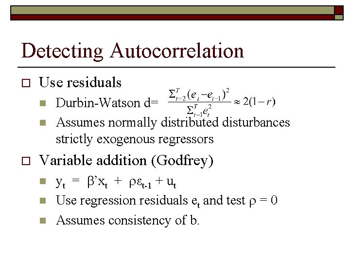
Detecting Autocorrelation o Use residuals n n o Durbin-Watson d= Assumes normally distributed disturbances strictly exogenous regressors Variable addition (Godfrey) n n n yt = ’xt + εt-1 + ut Use regression residuals et and test = 0 Assumes consistency of b.

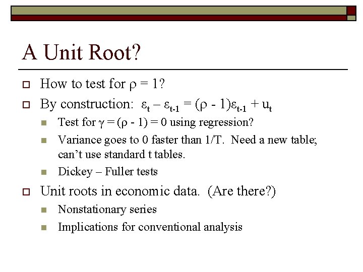
A Unit Root? o o How to test for = 1? By construction: εt – εt-1 = ( - 1)εt-1 + ut n n n o Test for γ = ( - 1) = 0 using regression? Variance goes to 0 faster than 1/T. Need a new table; can’t use standard t tables. Dickey – Fuller tests Unit roots in economic data. (Are there? ) n n Nonstationary series Implications for conventional analysis

Reinterpreting Autocorrelation

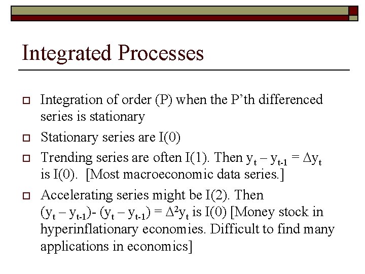
Integrated Processes o o Integration of order (P) when the P’th differenced series is stationary Stationary series are I(0) Trending series are often I(1). Then yt – yt-1 = yt is I(0). [Most macroeconomic data series. ] Accelerating series might be I(2). Then (yt – yt-1)- (yt – yt-1) = 2 yt is I(0) [Money stock in hyperinflationary economies. Difficult to find many applications in economics]

Real DPI and Real Consumption

Cointegration – Divergent Series?

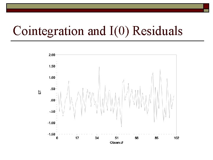
Cointegration o o o o X(t) and y(t) are obviously I(1) Looks like any linear combination of x(t) and y(t) will also be I(1) Does a model y(t) = bx(t) + u(u) where u(t) is I(0) make any sense? How can u(t) be I(0)? In fact, there is a linear combination, [1, - ] that is I(0). y(t) =. 1*t + noise, x(t) =. 2*t + noise y(t) and x(t) have a common trend y(t) and x(t) are cointegrated.

Cointegration and I(0) Residuals

The End