Econometrics Chengyuan Yin School of Mathematics Econometrics 19
![Computing the Asymptotic Variance We want to estimate {-E[H]}-1 Three ways: (1) Just compute Computing the Asymptotic Variance We want to estimate {-E[H]}-1 Three ways: (1) Just compute](https://slidetodoc.com/presentation_image_h2/b9466cea380902fa1b43f814b4e9b6de/image-26.jpg)
![Regression and Partial Effects +--------------+--------+--------+-----+ |Variable| Coefficient | Standard Error |b/St. Er. |P[|Z|>z]| Mean Regression and Partial Effects +--------------+--------+--------+-----+ |Variable| Coefficient | Standard Error |b/St. Er. |P[|Z|>z]| Mean](https://slidetodoc.com/presentation_image_h2/b9466cea380902fa1b43f814b4e9b6de/image-40.jpg)
![Comparison of Standard Errors +--------------+--------+--------+-----+ |Variable| Coefficient | Standard Error |b/St. Er. |P[|Z|>z]| Mean Comparison of Standard Errors +--------------+--------+--------+-----+ |Variable| Coefficient | Standard Error |b/St. Er. |P[|Z|>z]| Mean](https://slidetodoc.com/presentation_image_h2/b9466cea380902fa1b43f814b4e9b6de/image-41.jpg)
![LM Statistic --> --> calc ; beta 1=log(xbr(docvis)) $ matrix ; bmle 0=[beta 1/0/0/0] LM Statistic --> --> calc ; beta 1=log(xbr(docvis)) $ matrix ; bmle 0=[beta 1/0/0/0]](https://slidetodoc.com/presentation_image_h2/b9466cea380902fa1b43f814b4e9b6de/image-49.jpg)
- Slides: 49

Econometrics Chengyuan Yin School of Mathematics

Econometrics 19. Maximum Likelihood Estimation

Maximum Likelihood Estimation This defines a class of estimators based on the particular distribution assumed to have generated the observed random variable. The main advantage of ML estimators is that among all Consistent Asymptotically Normal Estimators, MLEs have optimal asymptotic properties. The main disadvantage is that they are not necessarily robust to failures of the distributional assumptions. They are very dependent on the particular assumptions. The oft cited disadvantage of their mediocre small sample properties is probably overstated in view of the usual paucity of viable alternatives.

Setting up the MLE The distribution of the observed random variable is written as a function of the parameters to be estimated P(yi|data, β) = Probability density | parameters. The likelihood function is constructed from the density Construction: Joint probability density function of the observed sample of data – generally the product when the data are a random sample.

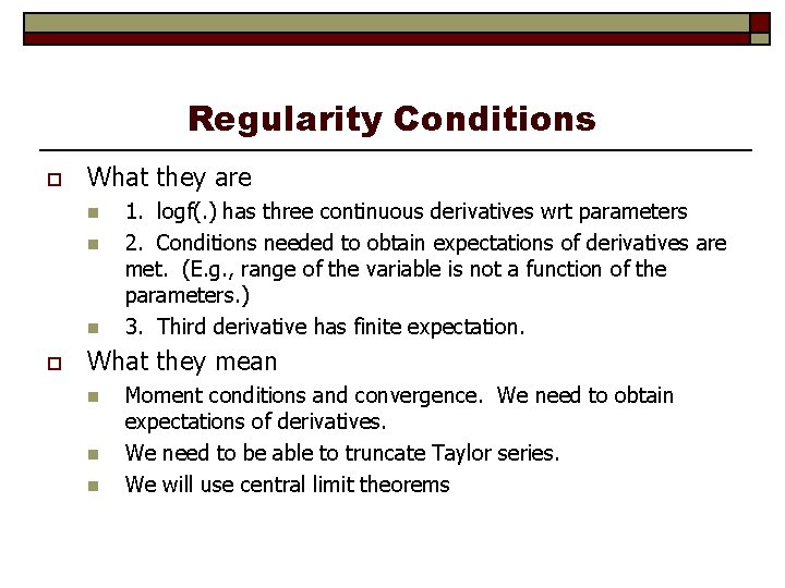
Regularity Conditions o What they are n n n o 1. logf(. ) has three continuous derivatives wrt parameters 2. Conditions needed to obtain expectations of derivatives are met. (E. g. , range of the variable is not a function of the parameters. ) 3. Third derivative has finite expectation. What they mean n Moment conditions and convergence. We need to obtain expectations of derivatives. We need to be able to truncate Taylor series. We will use central limit theorems

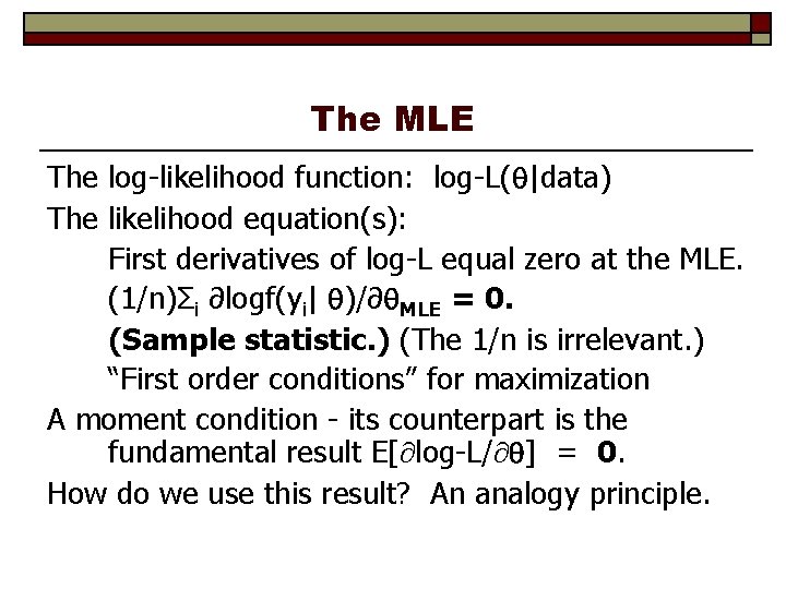
The MLE The log-likelihood function: log-L( |data) The likelihood equation(s): First derivatives of log-L equal zero at the MLE. (1/n)Σi ∂logf(yi| )/∂ MLE = 0. (Sample statistic. ) (The 1/n is irrelevant. ) “First order conditions” for maximization A moment condition - its counterpart is the fundamental result E[ log-L/ ] = 0. How do we use this result? An analogy principle.

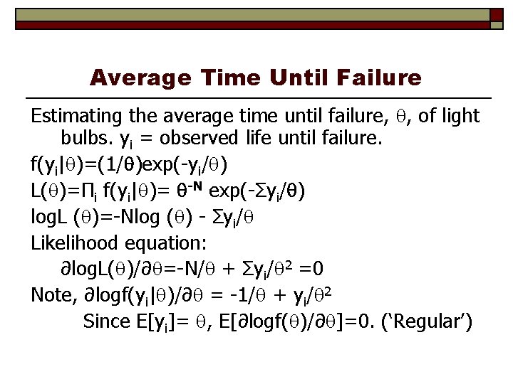
Average Time Until Failure Estimating the average time until failure, , of light bulbs. yi = observed life until failure. f(yi| )=(1/ )exp(-yi/ ) L( )=Πi f(yi| )= -N exp(-Σyi/ ) log. L ( )=-Nlog ( ) - Σyi/ Likelihood equation: ∂log. L( )/∂ =-N/ + Σyi/ 2 =0 Note, ∂logf(yi| )/∂ = -1/ + yi/ 2 Since E[yi]= , E[∂logf( )/∂ ]=0. (‘Regular’)

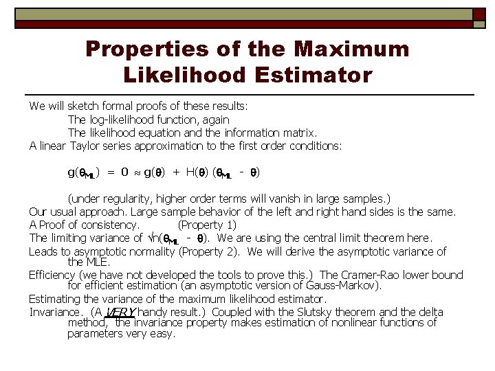
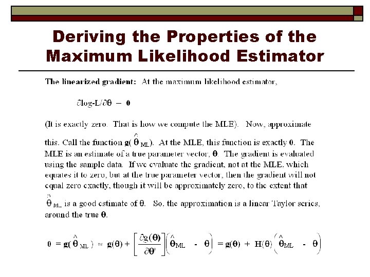
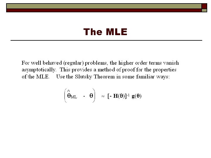
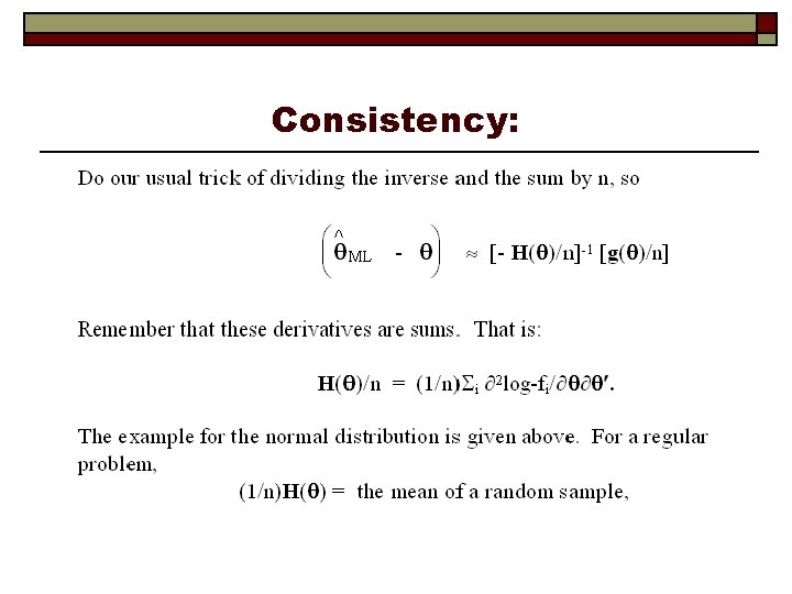
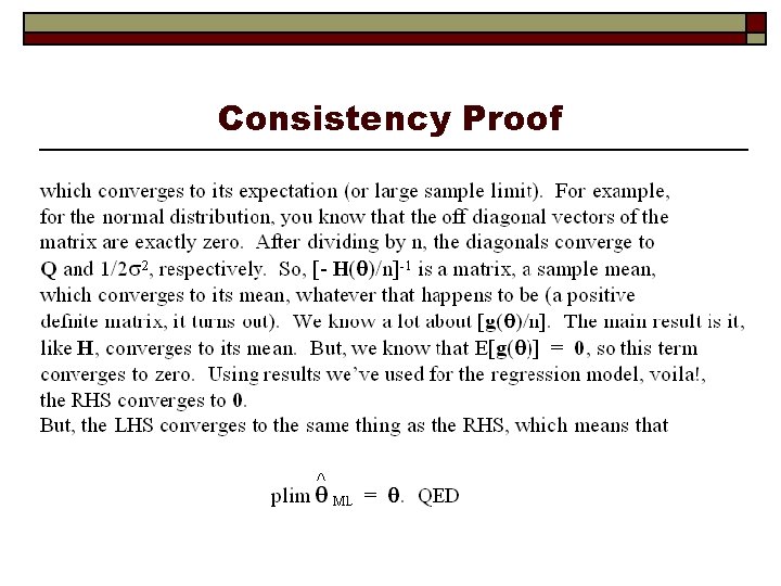
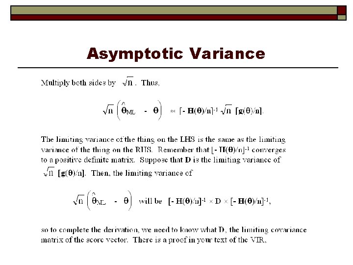
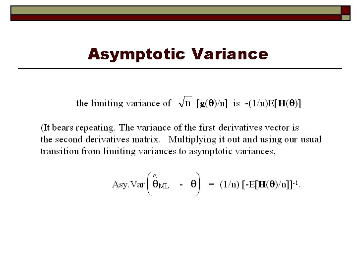
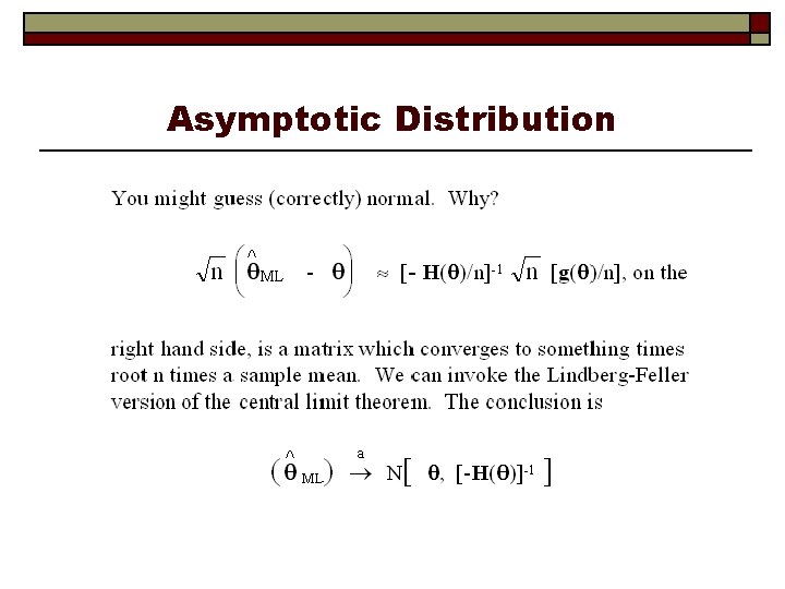
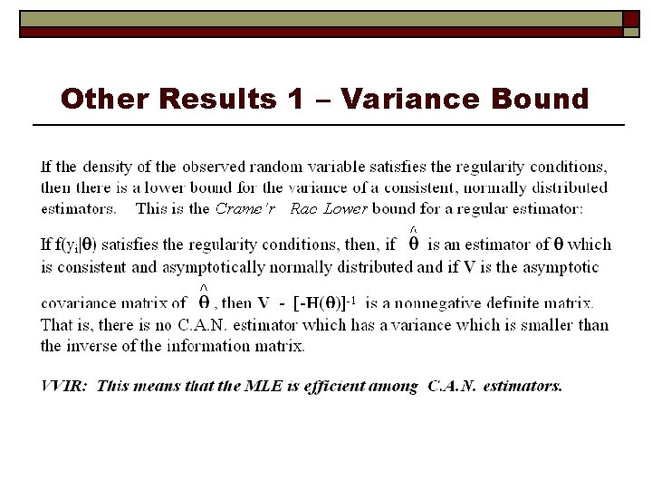
Properties of the Maximum Likelihood Estimator We will sketch formal proofs of these results: The log-likelihood function, again The likelihood equation and the information matrix. A linear Taylor series approximation to the first order conditions: g( ML) = 0 g( ) + H( ) ( ML - ) (under regularity, higher order terms will vanish in large samples. ) Our usual approach. Large sample behavior of the left and right hand sides is the same. A Proof of consistency. (Property 1) The limiting variance of n( ML - ). We are using the central limit theorem here. Leads to asymptotic normality (Property 2). We will derive the asymptotic variance of the MLE. Efficiency (we have not developed the tools to prove this. ) The Cramer-Rao lower bound for efficient estimation (an asymptotic version of Gauss-Markov). Estimating the variance of the maximum likelihood estimator. Invariance. (A VERY handy result. ) Coupled with the Slutsky theorem and the delta method, the invariance property makes estimation of nonlinear functions of parameters very easy.

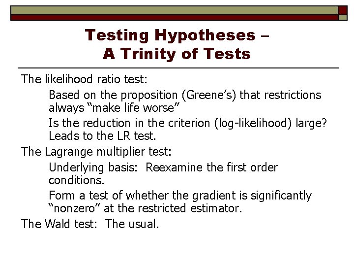
Testing Hypotheses – A Trinity of Tests The likelihood ratio test: Based on the proposition (Greene’s) that restrictions always “make life worse” Is the reduction in the criterion (log-likelihood) large? Leads to the LR test. The Lagrange multiplier test: Underlying basis: Reexamine the first order conditions. Form a test of whether the gradient is significantly “nonzero” at the restricted estimator. The Wald test: The usual.

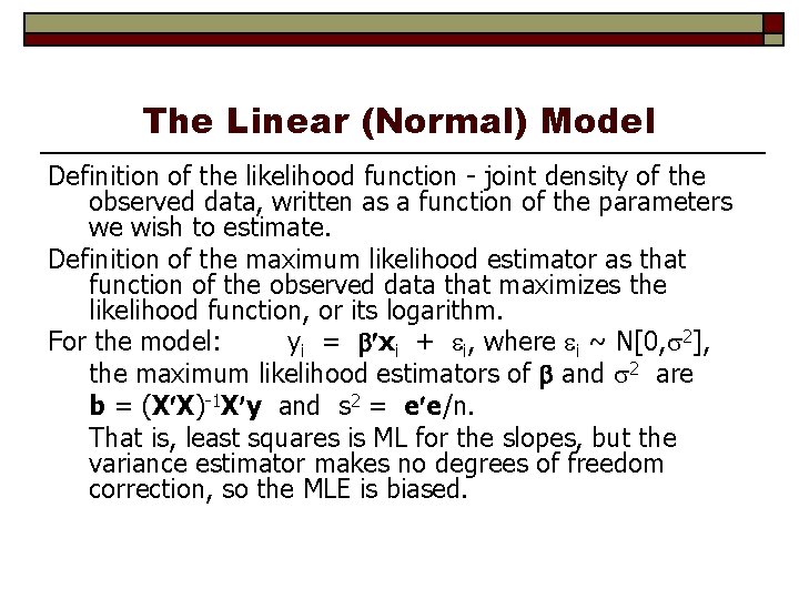
The Linear (Normal) Model Definition of the likelihood function - joint density of the observed data, written as a function of the parameters we wish to estimate. Definition of the maximum likelihood estimator as that function of the observed data that maximizes the likelihood function, or its logarithm. For the model: yi = xi + i, where i ~ N[0, 2], the maximum likelihood estimators of and 2 are b = (X X)-1 X y and s 2 = e e/n. That is, least squares is ML for the slopes, but the variance estimator makes no degrees of freedom correction, so the MLE is biased.

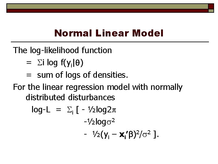
Normal Linear Model The log-likelihood function = i log f(yi| ) = sum of logs of densities. For the linear regression model with normally distributed disturbances log-L = i [ - ½log 2 - ½(yi – xi )2/ 2 ].

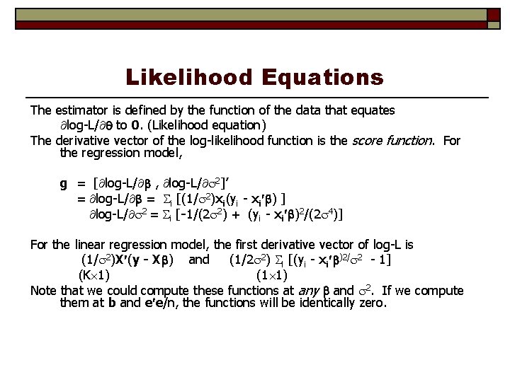
Likelihood Equations The estimator is defined by the function of the data that equates log-L/ to 0. (Likelihood equation) The derivative vector of the log-likelihood function is the score function. For the regression model, g = [ log-L/ , log-L/ 2]’ = log-L/ = i [(1/ 2)xi(yi - xi ) ] log-L/ 2 = i [-1/(2 2) + (yi - xi )2/(2 4)] For the linear regression model, the first derivative vector of log-L is (1/ 2)X (y - X ) and (1/2 2) i [(yi - xi )2/ 2 - 1] (K 1) (1 1) Note that we could compute these functions at any and 2. If we compute them at b and e e/n, the functions will be identically zero.

Moment Equations Note that g = i gi is a random vector and that each term in the sum has expectation zero. It follows that E[(1/n)g] = 0. Our estimator is found by finding the that sets the sample mean of the gs to 0. That is, theoretically, E[gi( , 2)] = 0. We find the estimator as that function which produces (1/n) i gi(b , s 2) = 0. Note the similarity to the way we would estimate any mean. If E[xi] = , then E[xi - ] = 0. We estimate by finding the function of the data that produces (1/n) i (xi - m) = 0, which is, of course the sample mean. There are two main components to the “regularity conditions for maximum likelihood estimation. The first is that the first derivative has expected value 0. That ‘moment equation’ motivates the MLE

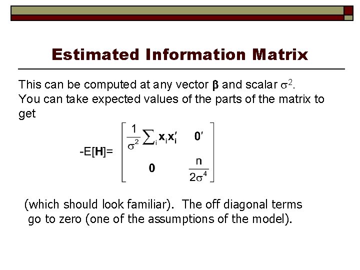
Information Matrix The negative of the second derivatives matrix of the log-likelihood, -H = is called the information matrix. It is usually a random matrix, also. For the linear regression model,

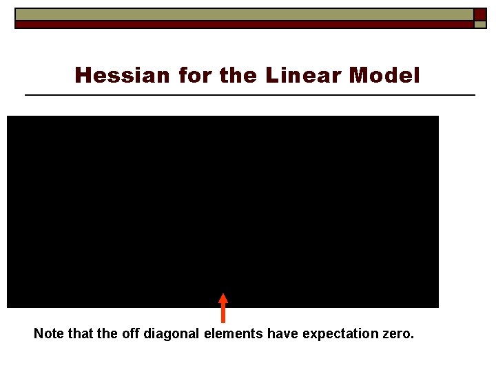
Hessian for the Linear Model Note that the off diagonal elements have expectation zero.

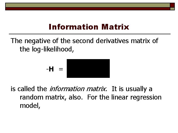
Estimated Information Matrix This can be computed at any vector and scalar 2. You can take expected values of the parts of the matrix to get (which should look familiar). The off diagonal terms go to zero (one of the assumptions of the model).

Deriving the Properties of the Maximum Likelihood Estimator

The MLE

Consistency:

Consistency Proof

Asymptotic Variance

Asymptotic Variance

Asymptotic Distribution

Other Results 1 – Variance Bound

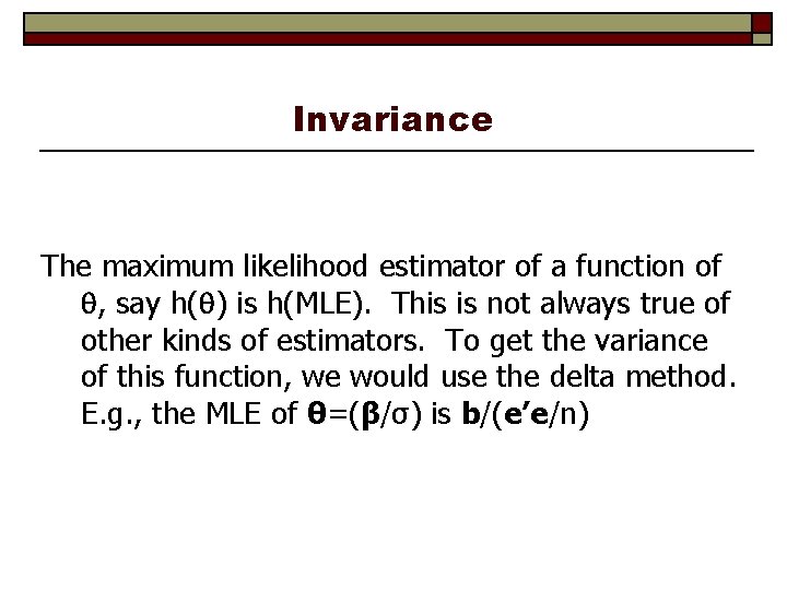
Invariance The maximum likelihood estimator of a function of , say h( ) is h(MLE). This is not always true of other kinds of estimators. To get the variance of this function, we would use the delta method. E. g. , the MLE of θ=(β/σ) is b/(e’e/n)
![Computing the Asymptotic Variance We want to estimate EH1 Three ways 1 Just compute Computing the Asymptotic Variance We want to estimate {-E[H]}-1 Three ways: (1) Just compute](https://slidetodoc.com/presentation_image_h2/b9466cea380902fa1b43f814b4e9b6de/image-26.jpg)
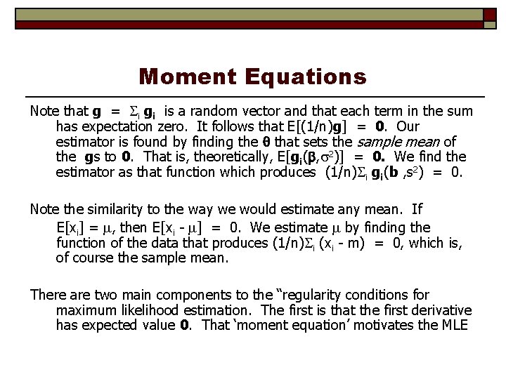
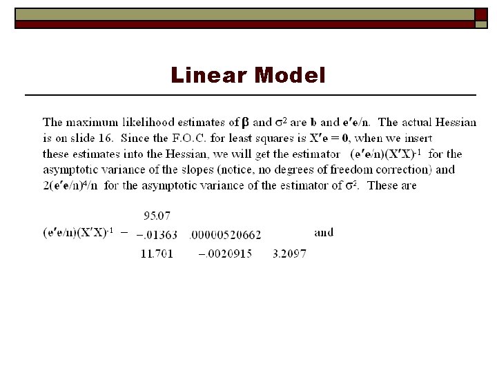
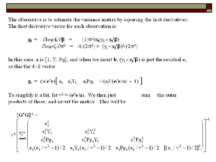
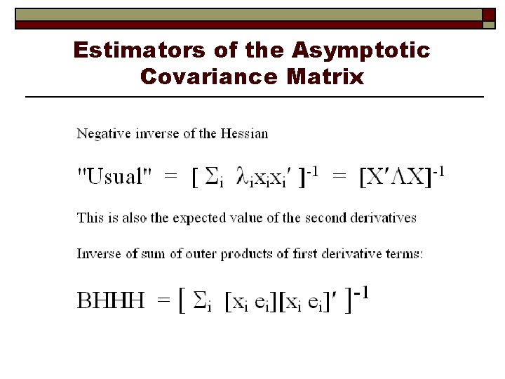
Computing the Asymptotic Variance We want to estimate {-E[H]}-1 Three ways: (1) Just compute the negative of the actual second derivatives matrix and invert it. (2) Insert the maximum likelihood estimates into the known expected values of the second derivatives matrix. Sometimes (1) and (2) give the same answer (for example, in the linear regression model). (3) Since E[H] is the variance of the first derivatives, estimate this with the sample variance (i. e. , mean square) of the first derivatives. This will almost always be different from (1) and (2). Since they are estimating the same thing, in large samples, all three will give the same answer. Current practice in econometrics often favors (3). Stata rarely uses (3). Others do.

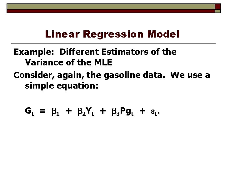
Linear Regression Model Example: Different Estimators of the Variance of the MLE Consider, again, the gasoline data. We use a simple equation: Gt = 1 + 2 Yt + 3 Pgt + t.

Linear Model


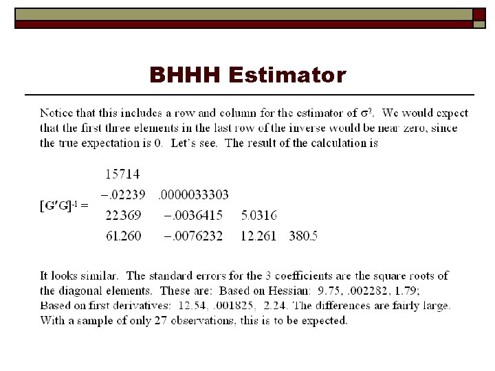
BHHH Estimator

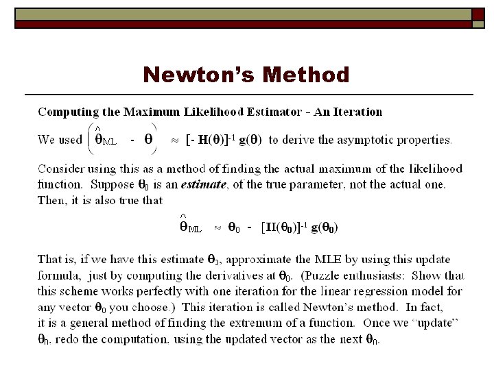
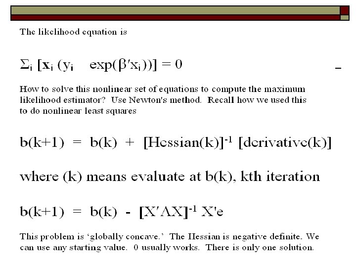
Newton’s Method

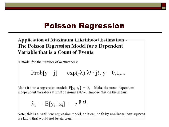
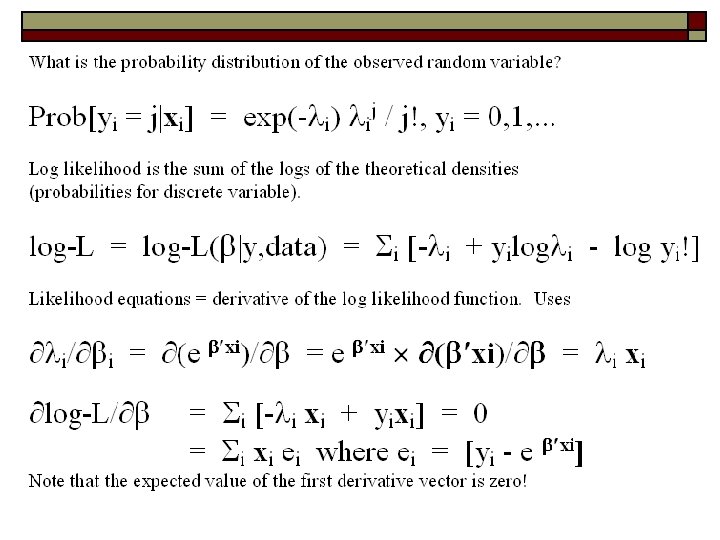
Poisson Regression


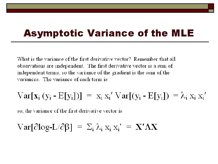
Asymptotic Variance of the MLE


Estimators of the Asymptotic Covariance Matrix

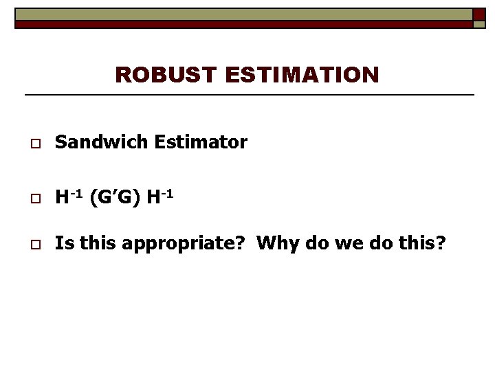
ROBUST ESTIMATION o Sandwich Estimator o H-1 (G’G) H-1 o Is this appropriate? Why do we do this?

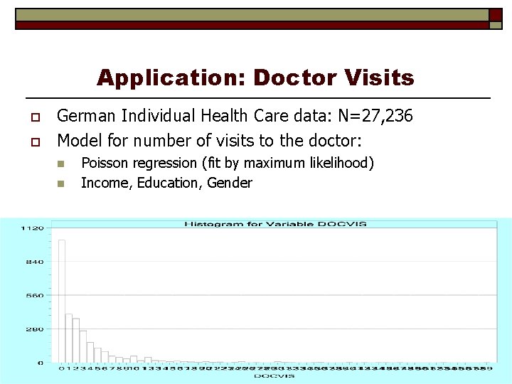
Application: Doctor Visits o o German Individual Health Care data: N=27, 236 Model for number of visits to the doctor: n n Poisson regression (fit by maximum likelihood) Income, Education, Gender

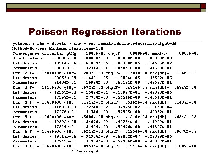
Poisson Regression Iterations poisson ; lhs = docvis ; rhs = one, female, hhninc, educ; mar; output=3$ Method=Newton; Maximum iterations=100 Convergence criteria: gt. Hg. 1000 D-05 chg. F. 0000 D+00 max|db|. 0000 D+00 Start values: . 00000 D+00 1 st derivs. -. 13214 D+06 -. 61899 D+05 -. 43338 D+05 -. 14596 D+07 Parameters: . 28002 D+01. 72374 D-01 -. 65451 D+00 -. 47608 D-01 Itr 2 F= -. 1587 D+06 gt. Hg=. 2832 D+03 chg. F=. 1587 D+06 max|db|=. 1346 D+01 1 st derivs. -. 33055 D+05 -. 14401 D+05 -. 10804 D+05 -. 36592 D+06 Parameters: . 21404 D+01. 16980 D+00 -. 60181 D+00 -. 48527 D-01 Itr 3 F= -. 1115 D+06 gt. Hg=. 9725 D+02 chg. F=. 4716 D+05 max|db|=. 6348 D+00 1 st derivs. -. 42953 D+04 -. 15074 D+04 -. 13927 D+04 -. 47823 D+05 Parameters: . 17997 D+01. 27758 D+00 -. 54519 D+00 -. 49513 D-01 Itr 4 F= -. 1063 D+06 gt. Hg=. 1545 D+02 chg. F=. 5162 D+04 max|db|=. 1437 D+00 1 st derivs. -. 11692 D+03 -. 22248 D+02 -. 37525 D+02 -. 13159 D+04 Parameters: . 17276 D+01. 31746 D+00 -. 52565 D+00 -. 49852 D-01 Itr 5 F= -. 1062 D+06 gt. Hg=. 5006 D+00 chg. F=. 1218 D+03 max|db|=. 6542 D-02 1 st derivs. -. 12522 D+00 -. 54690 D-02 -. 40254 D-01 -. 14232 D+01 Parameters: . 17249 D+01. 31954 D+00 -. 52476 D+00 -. 49867 D-01 Itr 6 F= -. 1062 D+06 gt. Hg=. 6215 D-03 chg. F=. 1254 D+00 max|db|=. 9678 D-05 1 st derivs. -. 19317 D-06 -. 94936 D-09 -. 62872 D-07 -. 22029 D-05 Parameters: . 17249 D+01. 31954 D+00 -. 52476 D+00 -. 49867 D-01 Itr 7 F= -. 1062 D+06 gt. Hg=. 9957 D-09 chg. F=. 1941 D-06 max|db|=. 1602 D-10 * Converged
![Regression and Partial Effects Variable Coefficient Standard Error bSt Er PZz Mean Regression and Partial Effects +--------------+--------+--------+-----+ |Variable| Coefficient | Standard Error |b/St. Er. |P[|Z|>z]| Mean](https://slidetodoc.com/presentation_image_h2/b9466cea380902fa1b43f814b4e9b6de/image-40.jpg)
Regression and Partial Effects +--------------+--------+--------+-----+ |Variable| Coefficient | Standard Error |b/St. Er. |P[|Z|>z]| Mean of X| +--------------+--------+--------+-----+ Constant| 1. 72492985. 02000568 86. 222. 0000 FEMALE |. 31954440. 00696870 45. 854. 0000. 47877479 HHNINC | -. 52475878. 02197021 -23. 885. 0000. 35208362 EDUC | -. 04986696. 00172872 -28. 846. 0000 11. 3206310 +----------------------+ | Partial derivatives of expected val. with | | respect to the vector of characteristics. | | Effects are averaged over individuals. | | Observations used for means are All Obs. | | Conditional Mean at Sample Point 3. 1835 | | Scale Factor for Marginal Effects 3. 1835 | +----------------------+ +--------------+--------+--------+-----+ |Variable| Coefficient | Standard Error |b/St. Er. |P[|Z|>z]| Mean of X| +--------------+--------+--------+-----+ Constant| 5. 49135704. 07890083 69. 598. 0000 FEMALE | 1. 01727755. 02427607 41. 905. 0000. 47877479 HHNINC | -1. 67058263. 07312900 -22. 844. 0000. 35208362 EDUC | -. 15875271. 00579668 -27. 387. 0000 11. 3206310
![Comparison of Standard Errors Variable Coefficient Standard Error bSt Er PZz Mean Comparison of Standard Errors +--------------+--------+--------+-----+ |Variable| Coefficient | Standard Error |b/St. Er. |P[|Z|>z]| Mean](https://slidetodoc.com/presentation_image_h2/b9466cea380902fa1b43f814b4e9b6de/image-41.jpg)
Comparison of Standard Errors +--------------+--------+--------+-----+ |Variable| Coefficient | Standard Error |b/St. Er. |P[|Z|>z]| Mean of X| +--------------+--------+--------+-----+ Constant| 1. 72492985. 02000568 86. 222. 0000 FEMALE |. 31954440. 00696870 45. 854. 0000. 47877479 HHNINC | -. 52475878. 02197021 -23. 885. 0000. 35208362 EDUC | -. 04986696. 00172872 -28. 846. 0000 11. 3206310 BHHH +--------------+--------+--------+ |Variable| Coefficient | Standard Error |b/St. Er. |P[|Z|>z]| +--------------+--------+--------+ Constant| 1. 72492985. 00677787 254. 495. 0000 FEMALE |. 31954440. 00217499 146. 918. 0000 HHNINC | -. 52475878. 00733328 -71. 559. 0000 EDUC | -. 04986696. 00062283 -80. 065. 0000 Why are they so different? Model failure. This is a panel. There is autocorrelation.

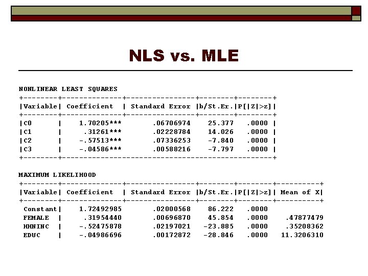
NLS vs. MLE NONLINEAR LEAST SQUARES +--------------+--------+--------+ |Variable| Coefficient | Standard Error |b/St. Er. |P[|Z|>z]| +--------------+--------+--------+ |C 0 | 1. 70205***. 06706974 25. 377. 0000 | |C 1 |. 31261***. 02228784 14. 026. 0000 | |C 2 | -. 57513***. 07336253 -7. 840. 0000 | |C 3 | -. 04586***. 00588216 -7. 797. 0000 | +-----------------------------+ MAXIMUM LIKELIHOOD +--------------+--------+--------+-----+ |Variable| Coefficient | Standard Error |b/St. Er. |P[|Z|>z]| Mean of X| +--------------+--------+--------+-----+ Constant| 1. 72492985. 02000568 86. 222. 0000 FEMALE |. 31954440. 00696870 45. 854. 0000. 47877479 HHNINC | -. 52475878. 02197021 -23. 885. 0000. 35208362 EDUC | -. 04986696. 00172872 -28. 846. 0000 11. 3206310

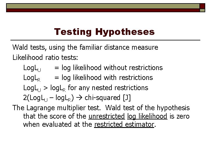
Testing Hypotheses Wald tests, using the familiar distance measure Likelihood ratio tests: Log. LU = log likelihood without restrictions Log. LR = log likelihood with restrictions Log. LU > log. LR for any nested restrictions 2(Log. LU – log. LR) chi-squared [J] The Lagrange multiplier test. Wald test of the hypothesis that the score of the unrestricted log likelihood is zero when evaluated at the restricted estimator.

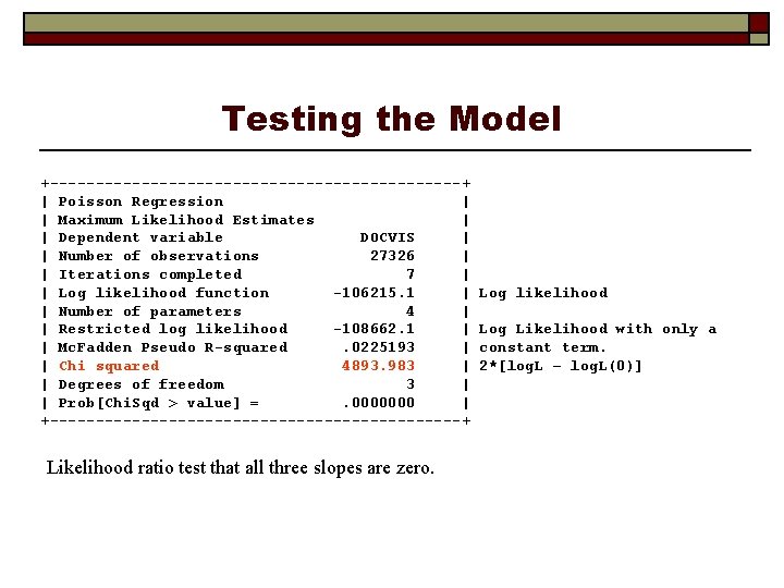
Testing the Model +-----------------------+ | Poisson Regression | | Maximum Likelihood Estimates | | Dependent variable DOCVIS | | Number of observations 27326 | | Iterations completed 7 | | Log likelihood function -106215. 1 | | Number of parameters 4 | | Restricted log likelihood -108662. 1 | | Mc. Fadden Pseudo R-squared. 0225193 | | Chi squared 4893. 983 | | Degrees of freedom 3 | | Prob[Chi. Sqd > value] =. 0000000 | +-----------------------+ Likelihood ratio test that all three slopes are zero. Log likelihood Log Likelihood with only a constant term. 2*[log. L – log. L(0)]

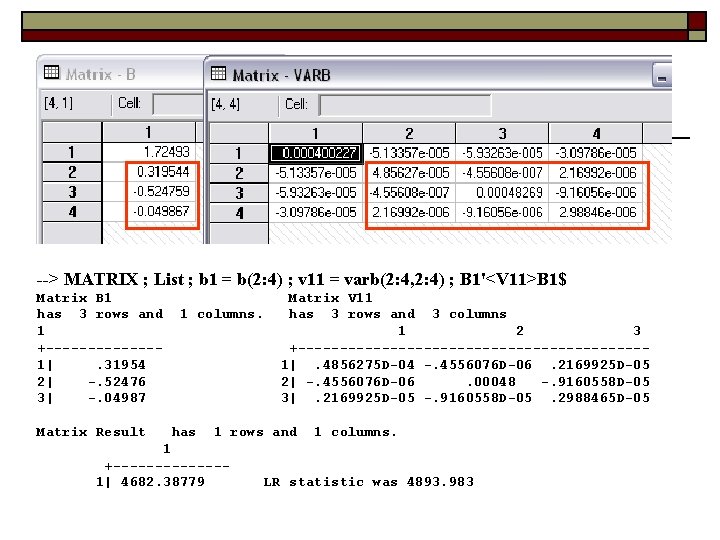
Wald Test --> MATRIX ; List ; b 1 = b(2: 4) ; v 11 = varb(2: 4, 2: 4) ; B 1'<V 11>B 1$ Matrix B 1 has 3 rows and 1 +-------1|. 31954 2| -. 52476 3| -. 04987 Matrix Result 1 columns. Matrix V 11 has 3 rows and 3 columns 1 2 3 +---------------------1|. 4856275 D-04 -. 4556076 D-06. 2169925 D-05 2| -. 4556076 D-06. 00048 -. 9160558 D-05 3|. 2169925 D-05 -. 9160558 D-05. 2988465 D-05 has 1 rows and 1 columns. 1 +-------1| 4682. 38779 LR statistic was 4893. 983

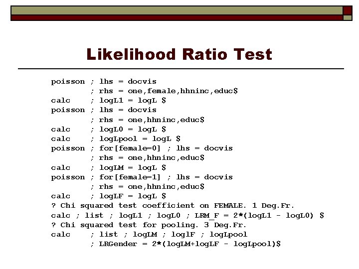
Likelihood Ratio Test poisson ; lhs = docvis ; rhs = one, female, hhninc, educ$ calc ; log. L 1 = log. L $ poisson ; lhs = docvis ; rhs = one, hhninc, educ$ calc ; log. L 0 = log. L $ calc ; log. Lpool = log. L $ poisson ; for[female=0] ; lhs = docvis ; rhs = one, hhninc, educ$ calc ; log. LM = log. L $ poisson ; for[female=1] ; lhs = docvis ; rhs = one, hhninc, educ$ calc ; log. LF = log. L $ ? Chi squared test coefficient on FEMALE. 1 Deg. Fr. calc ; list ; log. L 1 ; log. L 0 ; LRM_F = 2*(log. L 1 - log. L 0) $ ? Chi squared test for pooling. 3 Deg. Fr. calc ; list ; log. LM ; logl. F ; log. Lpool ; LRGender = 2*(log. LM+log. LF - log. Lpool)$

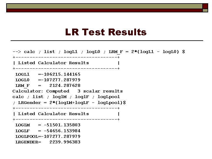
LR Test Results --> calc ; list ; log. L 1 ; log. L 0 ; LRM_F = 2*(log. L 1 - log. L 0) $ +------------------+ | Listed Calculator Results | +------------------+ LOGL 1 =-106215. 144165 LOGL 0 =-107277. 287979 LRM_F = 2124. 287628 Calculator: Computed 3 scalar results calc ; list ; logl. M ; logl. F ; log. Lpool ; LRGender = 2*(log. LM+log. LF - log. Lpool)$ +------------------+ | Listed Calculator Results | +------------------+ LOGLM = -51501. 135803 LOGLF = -54656. 153984 LOGLPOOL=-107277. 287979 LRGENDER= 2239. 996383

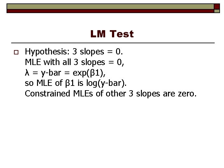
LM Test o Hypothesis: 3 slopes = 0. MLE with all 3 slopes = 0, λ = y-bar = exp(β 1), so MLE of β 1 is log(y-bar). Constrained MLEs of other 3 slopes are zero.
![LM Statistic calc beta 1logxbrdocvis matrix bmle 0beta 1000 LM Statistic --> --> calc ; beta 1=log(xbr(docvis)) $ matrix ; bmle 0=[beta 1/0/0/0]](https://slidetodoc.com/presentation_image_h2/b9466cea380902fa1b43f814b4e9b6de/image-49.jpg)
LM Statistic --> --> calc ; beta 1=log(xbr(docvis)) $ matrix ; bmle 0=[beta 1/0/0/0] $ create ; lambda 0 = exp(x'bmle 0) ; res 0 = docvis - lambda 0 $ matrix ; list ; g 0 = x'res 0 ; h 0 = x'[lambda 0]x ; lm = g 0'*<h 0>*g 0$ Matrix G 0 has 4 rows and 1 columns. +-------1|. 2664385 D-08 2| 7944. 94441 3|-1781. 12219 4| -. 3062440 D+05 Matrix H 0 has 4 rows and 4 columns. +----------------------------1|. 8699300 D+05. 4165006 D+05. 3062881 D+05. 9848157 D+06 2|. 4165006 D+05. 1434824 D+05. 4530019 D+06 3|. 3062881 D+05. 1434824 D+05. 1350638 D+05. 3561238 D+06 4|. 9848157 D+06. 4530019 D+06. 3561238 D+06. 1161892 D+08 Matrix LM has 1 rows and 1 columns. +-------1| 4715. 41008 Wald was 4682. 38779 LR statistic was 4893. 983