Econometrics Chengyuan Yin School of Mathematics Econometrics 16
![Finding Heteroscedasticity The central issue is whether E[ 2] = 2 i is related Finding Heteroscedasticity The central issue is whether E[ 2] = 2 i is related](https://slidetodoc.com/presentation_image_h2/68936b3ddb531c67eb4a5fb184a42e47/image-12.jpg)
![Newey-West +--------------+--------+---------+-----+ |Variable | Coefficient | Standard Error |t-ratio |P[|T|>t] | Mean of X| Newey-West +--------------+--------+---------+-----+ |Variable | Coefficient | Standard Error |t-ratio |P[|T|>t] | Mean of X|](https://slidetodoc.com/presentation_image_h2/68936b3ddb531c67eb4a5fb184a42e47/image-25.jpg)
- Slides: 26

Econometrics Chengyuan Yin School of Mathematics

Econometrics 16. Applications of the Generalized Regression Model

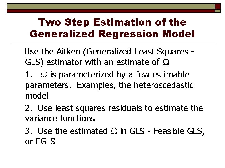
Two Step Estimation of the Generalized Regression Model Use the Aitken (Generalized Least Squares GLS) estimator with an estimate of 1. is parameterized by a few estimable parameters. Examples, the heteroscedastic model 2. Use least squares residuals to estimate the variance functions 3. Use the estimated in GLS - Feasible GLS, or FGLS

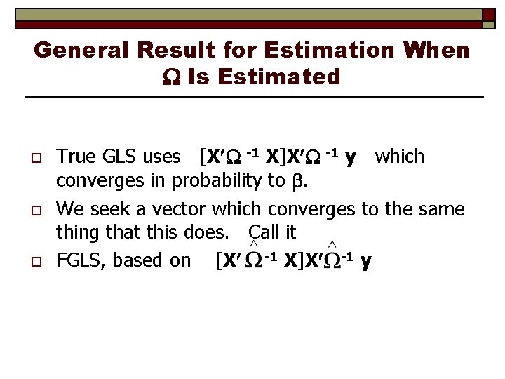
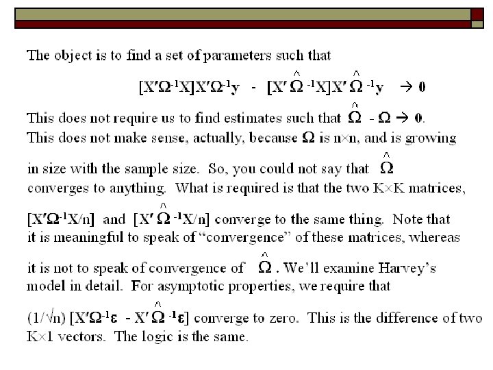
General Result for Estimation When Is Estimated o o o True GLS uses [X -1 X]X -1 y which converges in probability to . We seek a vector which converges to the same thing that this does. Call it FGLS, based on [X -1 X]X -1 y


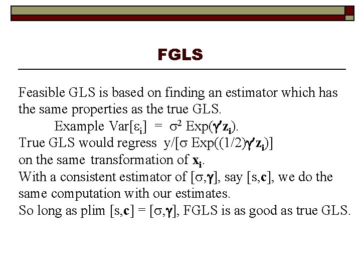
FGLS Feasible GLS is based on finding an estimator which has the same properties as the true GLS. Example Var[ i] = 2 Exp( zi). True GLS would regress y/[ Exp((1/2) zi)] on the same transformation of xi. With a consistent estimator of [ , ], say [s, c], we do the same computation with our estimates. So long as plim [s, c] = [ , ], FGLS is as good as true GLS.

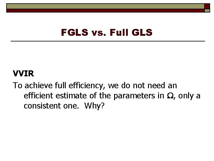
FGLS vs. Full GLS VVIR To achieve full efficiency, we do not need an efficient estimate of the parameters in , only a consistent one. Why?

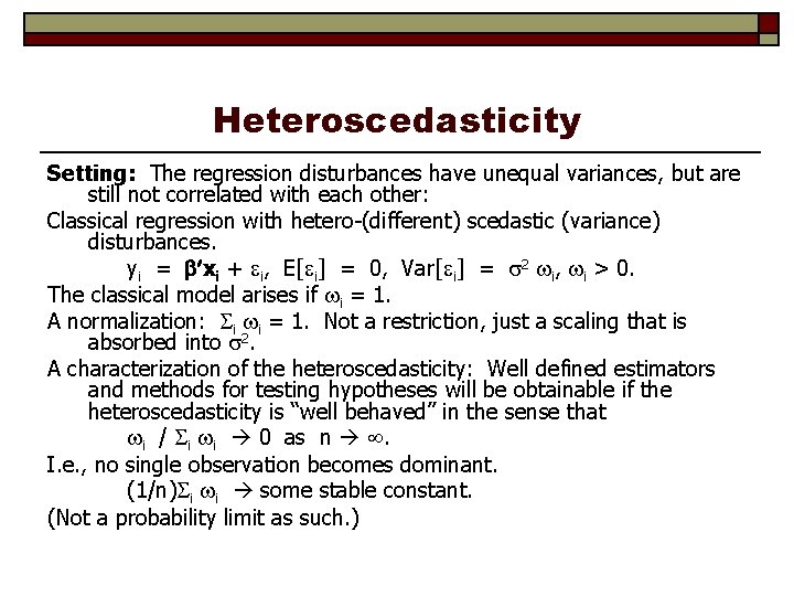
Heteroscedasticity Setting: The regression disturbances have unequal variances, but are still not correlated with each other: Classical regression with hetero-(different) scedastic (variance) disturbances. yi = xi + i, E[ i] = 0, Var[ i] = 2 i, i > 0. The classical model arises if i = 1. A normalization: i i = 1. Not a restriction, just a scaling that is absorbed into 2. A characterization of the heteroscedasticity: Well defined estimators and methods for testing hypotheses will be obtainable if the heteroscedasticity is “well behaved” in the sense that i / i i 0 as n . I. e. , no single observation becomes dominant. (1/n) i i some stable constant. (Not a probability limit as such. )

GR Model and Testing Implications for conventional estimation technique and hypothesis testing: 1. b is still unbiased. Proof of unbiasedness did not rely on homoscedasticity 2. Consistent? We need the more general proof. Not difficult. 3. If plim b = , then plim s 2 = 2 (with the normalization).

Inference Based on OLS What of s 2(X X)-1 ? Depends on X X - X X. If they are nearly the same, the OLS covariance matrix is OK. When will they be nearly the same? Relates to an interesting property of weighted averages. Suppose i is randomly drawn from a distribution with E[ i] = 1. Then, (1/n) i i xi 2 E[x 2], just like (1/n) i xi 2. This is the crux of the discussion in your text.

Inference Based on OLS VIR: For the heteroscedasticity to be substantive wrt estimation and inference by LS, the weights must be correlated with xs and/or their squares. (Text, page 220. ) More likely, the heteroscedasticity will be important. Then, b is inefficient. (Later) The White estimator. ROBUST estimation of the variance of b. Implication for testing hypotheses. We will use Wald tests. Why? (ROBUST TEST STATISTICS)
![Finding Heteroscedasticity The central issue is whether E 2 2 i is related Finding Heteroscedasticity The central issue is whether E[ 2] = 2 i is related](https://slidetodoc.com/presentation_image_h2/68936b3ddb531c67eb4a5fb184a42e47/image-12.jpg)
Finding Heteroscedasticity The central issue is whether E[ 2] = 2 i is related to the xs or their squares in the model. Suggests an obvious strategy. Use residuals to estimate disturbances and look for relationships between ei 2 and xi and/or xi 2. For example, regressions of squared residuals on xs and their squares.

Procedures White’s general test: n. R 2 in the regression of ei 2 on all unique xs, squares, and cross products. Chi-squared[P] Breusch and Pagan’s Lagrange multiplier test. Regress [ei 2 /(e e/n) – 1] on Z (may be X). Chi-squared. Is n. R 2 with degrees of freedom rank of Z. (Very elegant. ) Others described in text for other purposes. E. g. , groupwise heteroscedasticity. Wald, LM, and LR tests all examine the dispersion of group specific least squares residual variances.

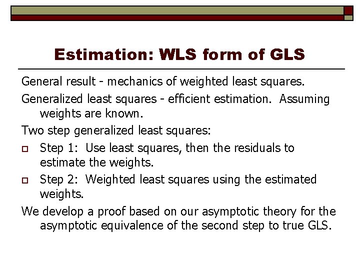
Estimation: WLS form of GLS General result - mechanics of weighted least squares. Generalized least squares - efficient estimation. Assuming weights are known. Two step generalized least squares: o Step 1: Use least squares, then the residuals to estimate the weights. o Step 2: Weighted least squares using the estimated weights. We develop a proof based on our asymptotic theory for the asymptotic equivalence of the second step to true GLS.

Autocorrelation The analysis of “autocorrelation” in the narrow sense of correlation of the disturbances across time largely parallels the discussions we’ve already done for the GR model in general and for heteroscedasticity in particular. One difference is that the relatively crisp results for the model of heteroscedasticity are replaced with relatively fuzzy, somewhat imprecise results here. The reason is that it is much more difficult to characterize meaningfully “well behaved” data in a time series context. Thus, for example, in contrast to the sharp result that produces the White robust estimator, theory underlying the Newey-West robust estimator is somewhat ambiguous in its requirement of a bland statement about “how far one must go back in time until correlation becomes unimportant. ”

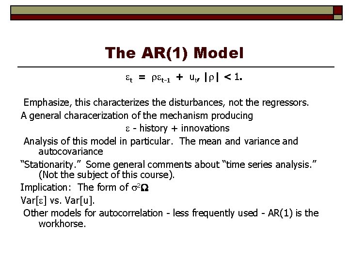
The AR(1) Model t = t-1 + ut, | | < 1. Emphasize, this characterizes the disturbances, not the regressors. A general characerization of the mechanism producing - history + innovations Analysis of this model in particular. The mean and variance and autocovariance “Stationarity. ” Some general comments about “time series analysis. ” (Not the subject of this course). Implication: The form of 2 Var[ ] vs. Var[u]. Other models for autocorrelation - less frequently used - AR(1) is the workhorse.

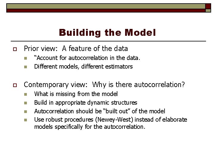
Building the Model o Prior view: A feature of the data n n o “Account for autocorrelation in the data. Different models, different estimators Contemporary view: Why is there autocorrelation? n n What is missing from the model Build in appropriate dynamic structures Autocorrelation should be “built out” of the model Use robust procedures (Newey-West) instead of elaborate models specifically for the autocorrelation.

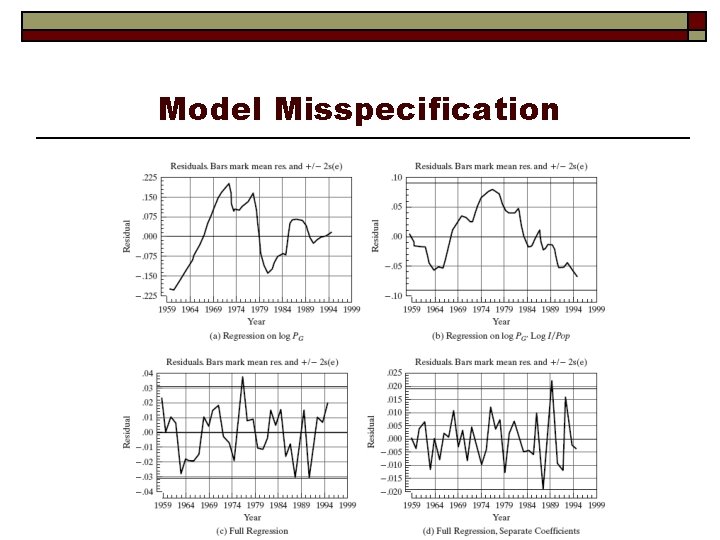
Model Misspecification

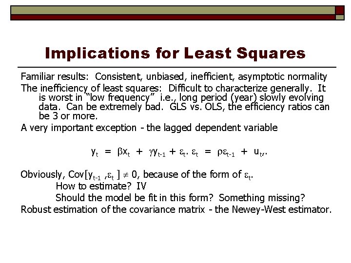
Implications for Least Squares Familiar results: Consistent, unbiased, inefficient, asymptotic normality The inefficiency of least squares: Difficult to characterize generally. It is worst in “low frequency” i. e. , long period (year) slowly evolving data. Can be extremely bad. GLS vs. OLS, the efficiency ratios can be 3 or more. A very important exception - the lagged dependent variable yt = xt + yt-1 + t. t = t-1 + ut, . Obviously, Cov[yt-1 , t ] 0, because of the form of t. How to estimate? IV Should the model be fit in this form? Something missing? Robust estimation of the covariance matrix - the Newey-West estimator.

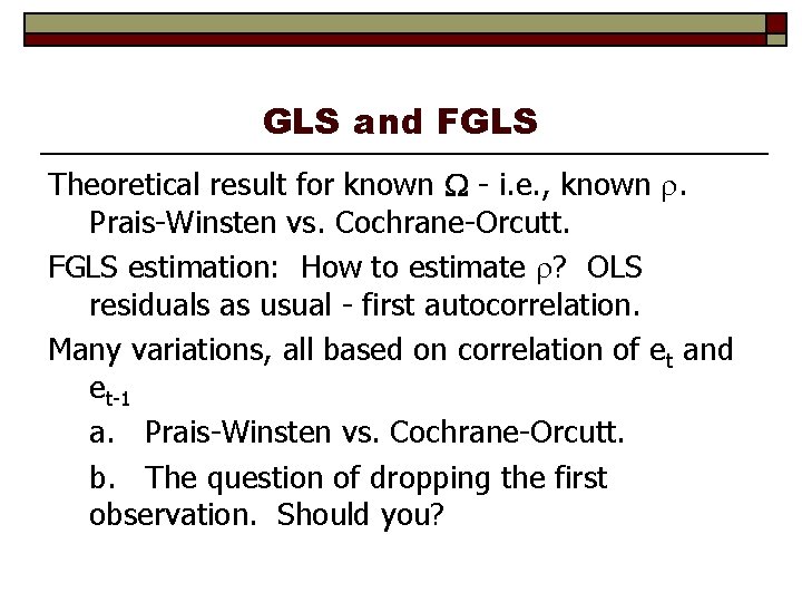
GLS and FGLS Theoretical result for known - i. e. , known . Prais-Winsten vs. Cochrane-Orcutt. FGLS estimation: How to estimate ? OLS residuals as usual - first autocorrelation. Many variations, all based on correlation of et and et-1 a. Prais-Winsten vs. Cochrane-Orcutt. b. The question of dropping the first observation. Should you?

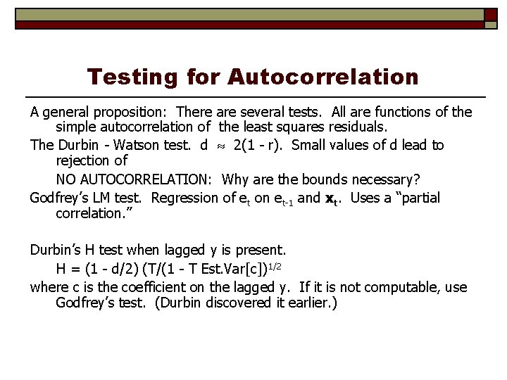
Testing for Autocorrelation A general proposition: There are several tests. All are functions of the simple autocorrelation of the least squares residuals. The Durbin - Watson test. d 2(1 - r). Small values of d lead to rejection of NO AUTOCORRELATION: Why are the bounds necessary? Godfrey’s LM test. Regression of et on et-1 and xt. Uses a “partial correlation. ” Durbin’s H test when lagged y is present. H = (1 - d/2) (T/(1 - T Est. Var[c])1/2 where c is the coefficient on the lagged y. If it is not computable, use Godfrey’s test. (Durbin discovered it earlier. )

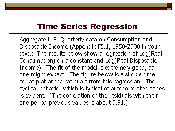
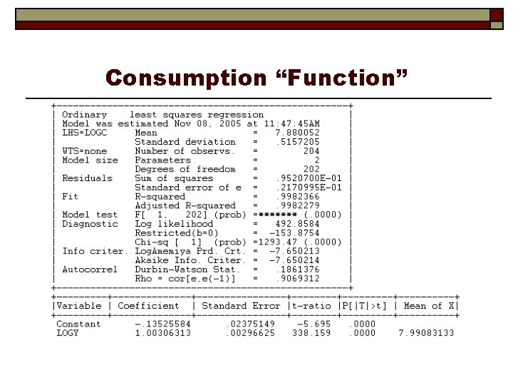
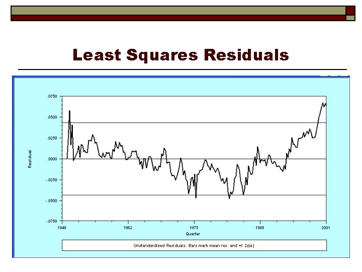
Time Series Regression Aggregate U. S. Quarterly data on Consumption and Disposable Income (Appendix F 5. 1, 1950 -2000 in your text. ) The results below show a regression of Log(Real Consumption) on a constant and Log(Real Disposable Income). The fit of the model is extremely good, as one might expect. The figure below is a simple time series plot of the residuals from this regression. The cyclical behavior which is typical of autocorrelated series is evident. (The correlation of the residuals with their one period previous values is about 0. 91. )

Consumption “Function”

Least Squares Residuals
![NeweyWest Variable Coefficient Standard Error tratio PTt Mean of X Newey-West +--------------+--------+---------+-----+ |Variable | Coefficient | Standard Error |t-ratio |P[|T|>t] | Mean of X|](https://slidetodoc.com/presentation_image_h2/68936b3ddb531c67eb4a5fb184a42e47/image-25.jpg)
Newey-West +--------------+--------+---------+-----+ |Variable | Coefficient | Standard Error |t-ratio |P[|T|>t] | Mean of X| +--------------+--------+---------+-----+ Constant -. 13525584. 02375149 -5. 695. 0000 LOGY 1. 00306313. 00296625 338. 159. 0000 7. 99083133 +--------------+--------+---------+-----+ |Variable | Coefficient | Standard Error |t-ratio |P[|T|>t] | Mean of X| +--------------+--------+---------+-----+ Constant -. 13525584. 07257279 -1. 864. 0638 LOGY 1. 00306313. 00938791 106. 846. 0000 7. 99083133

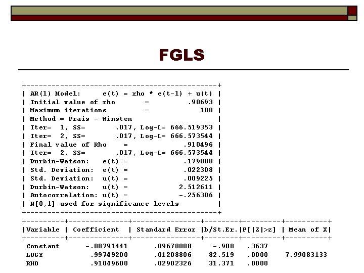
FGLS +-----------------------+ | AR(1) Model: e(t) = rho * e(t-1) + u(t) | | Initial value of rho =. 90693 | | Maximum iterations = 100 | | Method = Prais - Winsten | | Iter= 1, SS=. 017, Log-L= 666. 519353 | | Iter= 2, SS=. 017, Log-L= 666. 573544 | | Final value of Rho =. 910496 | | Iter= 2, SS=. 017, Log-L= 666. 573544 | | Durbin-Watson: e(t) =. 179008 | | Std. Deviation: e(t) =. 022308 | | Std. Deviation: u(t) =. 009225 | | Durbin-Watson: u(t) = 2. 512611 | | Autocorrelation: u(t) = -. 256306 | | N[0, 1] used for significance levels | +-----------------------+ +--------------+--------+---------+-----+ |Variable | Coefficient | Standard Error |b/St. Er. |P[|Z|>z] | Mean of X| +--------------+--------+---------+-----+ Constant -. 08791441. 09678008 -. 908. 3637 LOGY. 99749200. 01208806 82. 519. 0000 7. 99083133 RHO. 91049600. 02902326 31. 371. 0000