Econometrics Chengyuan Yin School of Mathematics Econometrics 22

Econometrics Chengyuan Yin School of Mathematics

Econometrics 22. The Generalized Method of Moments

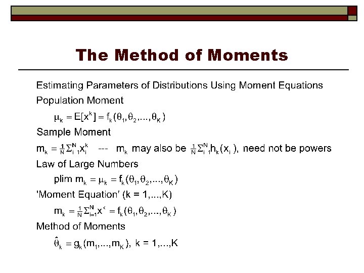
The Method of Moments

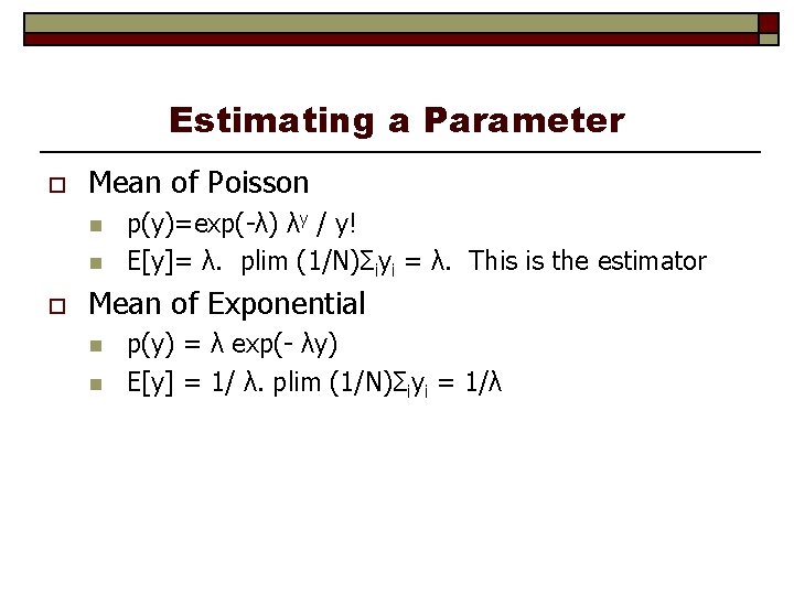
Estimating a Parameter o Mean of Poisson n n o p(y)=exp(-λ) λy / y! E[y]= λ. plim (1/N)Σiyi = λ. This is the estimator Mean of Exponential n n p(y) = λ exp(- λy) E[y] = 1/ λ. plim (1/N)Σiyi = 1/λ

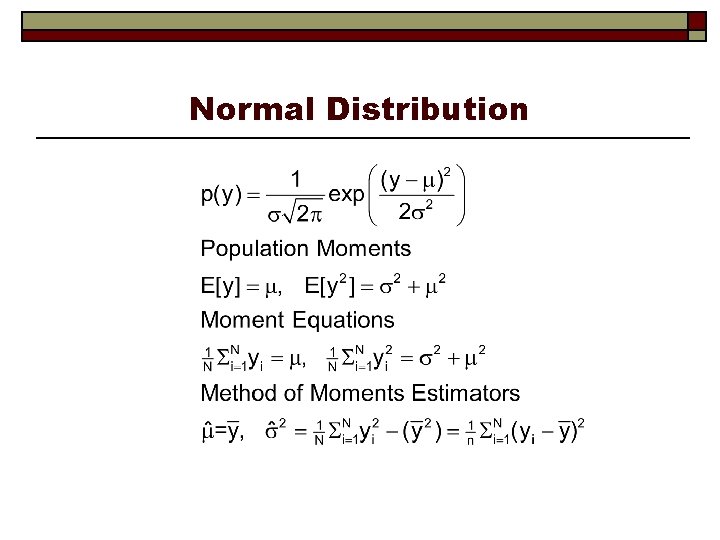
Normal Distribution

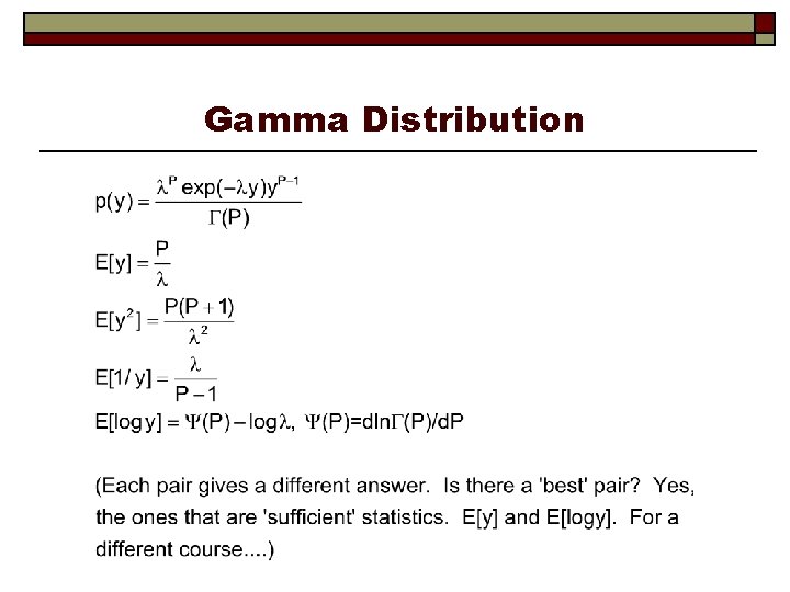
Gamma Distribution

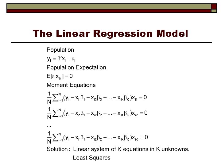
The Linear Regression Model

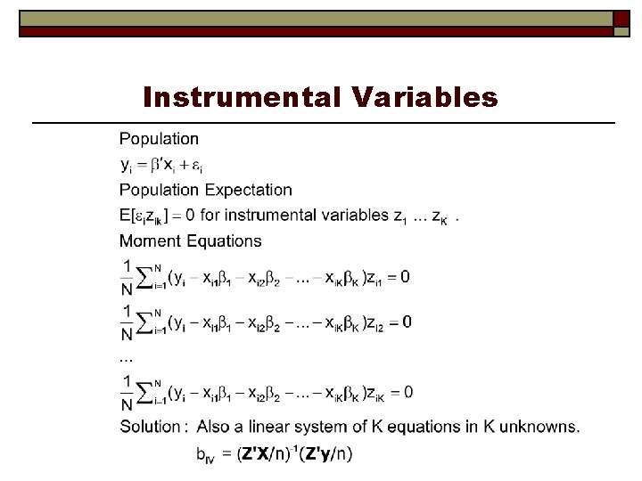
Instrumental Variables

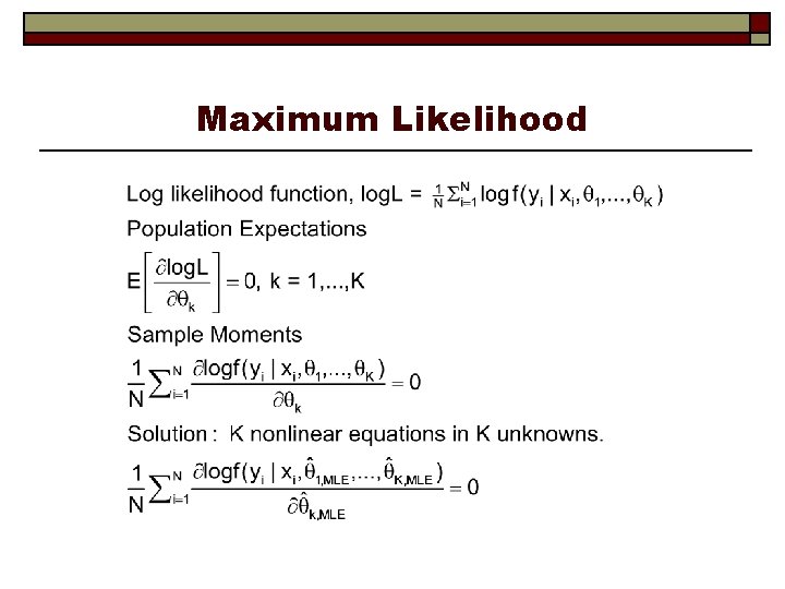
Maximum Likelihood

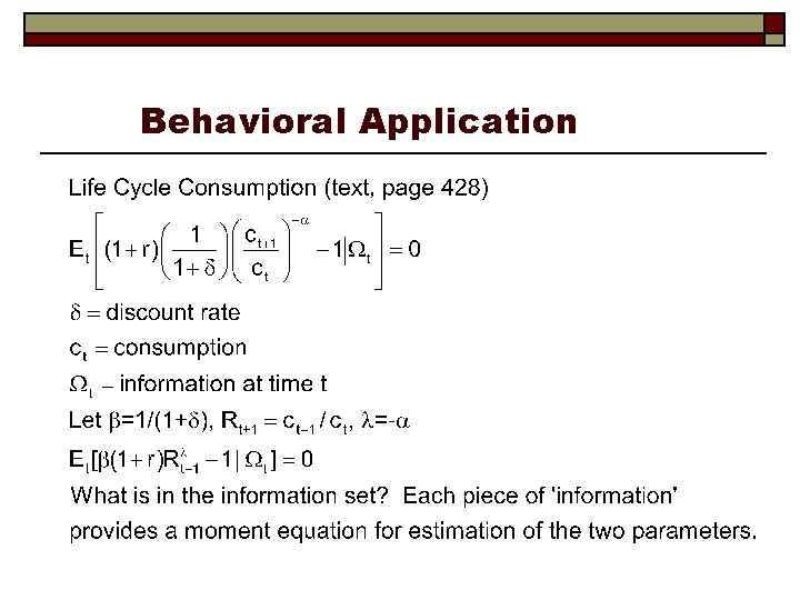
Behavioral Application

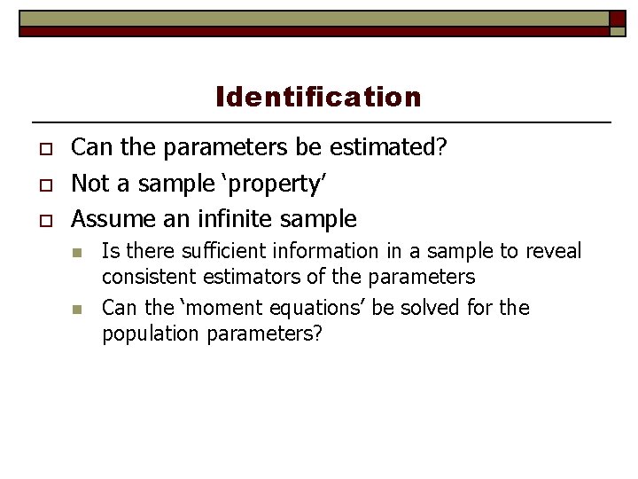
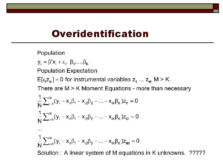
Identification o o o Can the parameters be estimated? Not a sample ‘property’ Assume an infinite sample n n Is there sufficient information in a sample to reveal consistent estimators of the parameters Can the ‘moment equations’ be solved for the population parameters?

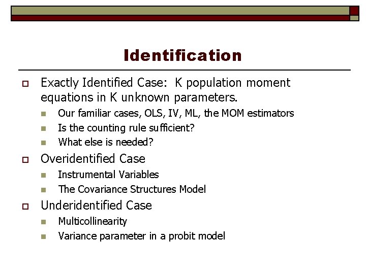
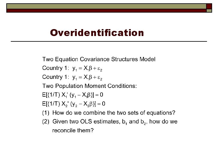
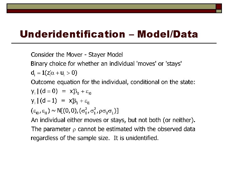
Identification o Exactly Identified Case: K population moment equations in K unknown parameters. n n n o Overidentified Case n n o Our familiar cases, OLS, IV, ML, the MOM estimators Is the counting rule sufficient? What else is needed? Instrumental Variables The Covariance Structures Model Underidentified Case n n Multicollinearity Variance parameter in a probit model

Overidentification

Overidentification

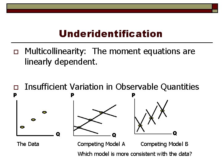
Underidentification o Multicollinearity: The moment equations are linearly dependent. o Insufficient Variation in Observable Quantities P P Q The Data P Q Competing Model A Q Competing Model B Which model is more consistent with the data?

Underidentification – Model/Data

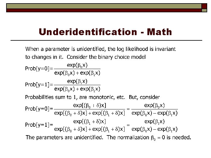
Underidentification - Math

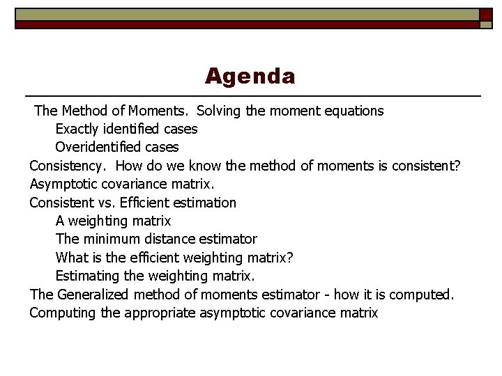
Agenda The Method of Moments. Solving the moment equations Exactly identified cases Overidentified cases Consistency. How do we know the method of moments is consistent? Asymptotic covariance matrix. Consistent vs. Efficient estimation A weighting matrix The minimum distance estimator What is the efficient weighting matrix? Estimating the weighting matrix. The Generalized method of moments estimator - how it is computed. Computing the appropriate asymptotic covariance matrix

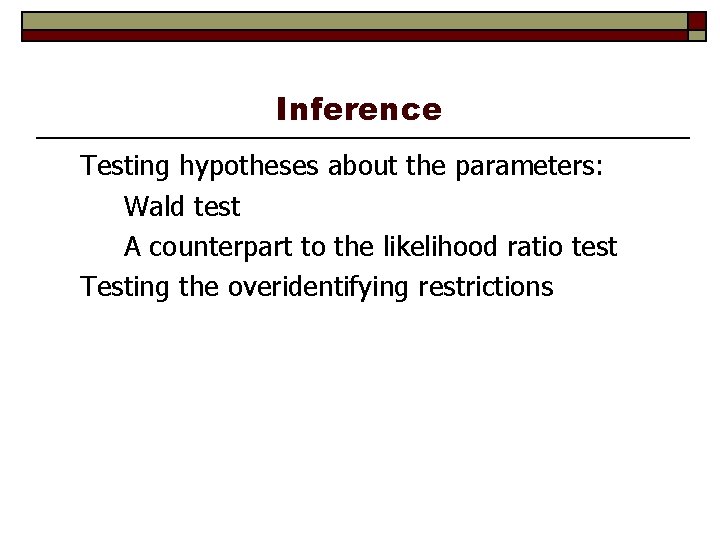
Inference Testing hypotheses about the parameters: Wald test A counterpart to the likelihood ratio test Testing the overidentifying restrictions

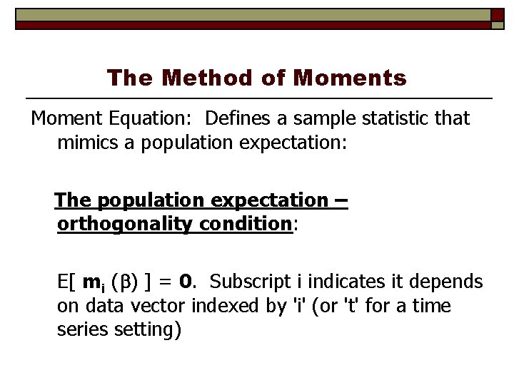
The Method of Moments Moment Equation: Defines a sample statistic that mimics a population expectation: The population expectation – orthogonality condition: E[ mi ( ) ] = 0. Subscript i indicates it depends on data vector indexed by 'i' (or 't' for a time series setting)

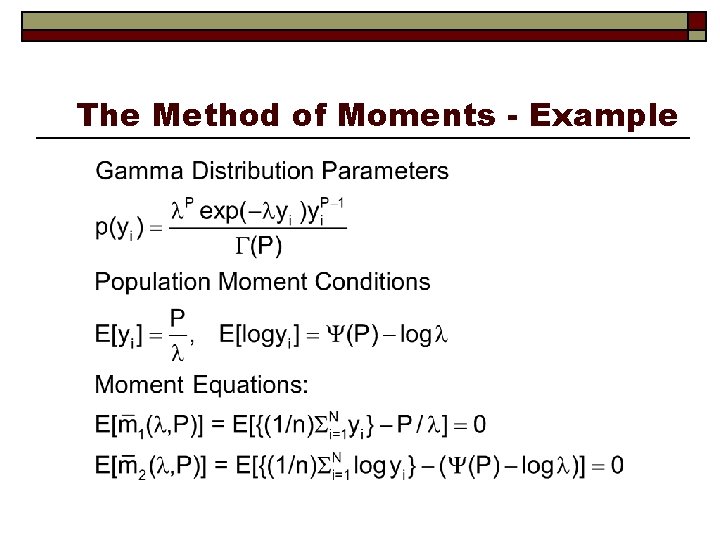
The Method of Moments - Example

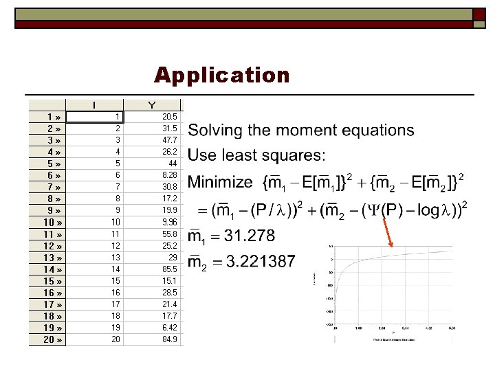
Application

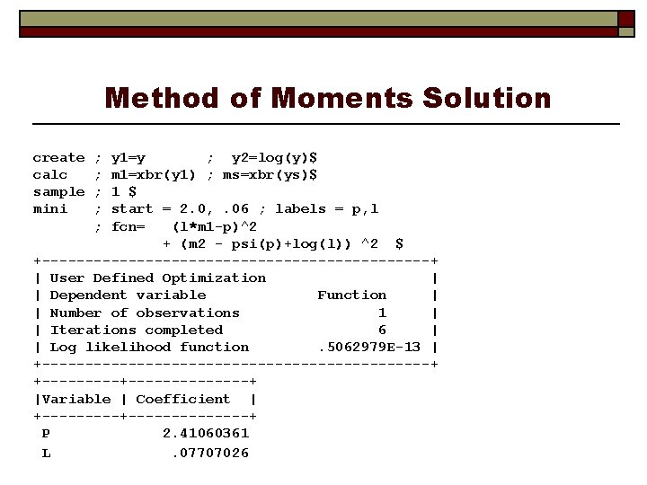
Method of Moments Solution create calc sample mini ; ; ; y 1=y ; y 2=log(y)$ m 1=xbr(y 1) ; ms=xbr(ys)$ 1 $ start = 2. 0, . 06 ; labels = p, l fcn= (l*m 1 -p)^2 + (m 2 - psi(p)+log(l)) ^2 $ +-----------------------+ | User Defined Optimization | | Dependent variable Function | | Number of observations 1 | | Iterations completed 6 | | Log likelihood function. 5062979 E-13 | +-----------------------+ +--------------+ |Variable | Coefficient | +--------------+ P 2. 41060361 L. 07707026

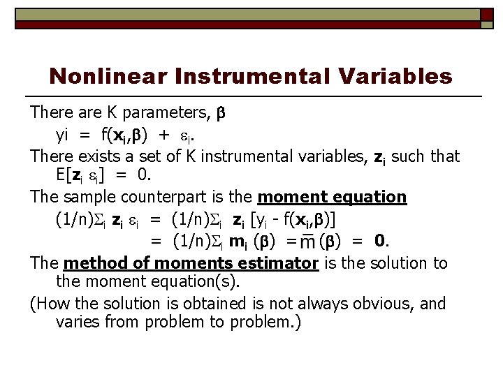
Nonlinear Instrumental Variables There are K parameters, yi = f(xi, ) + i. There exists a set of K instrumental variables, zi such that E[zi i] = 0. The sample counterpart is the moment equation (1/n) i zi i = (1/n) i zi [yi - f(xi, )] = (1/n) i mi ( ) = 0. The method of moments estimator is the solution to the moment equation(s). (How the solution is obtained is not always obvious, and varies from problem to problem. )

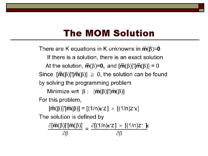
The MOM Solution

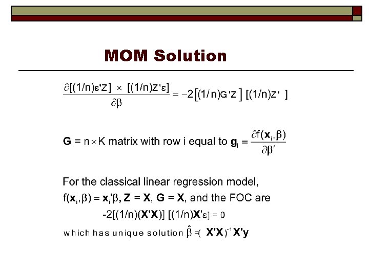
MOM Solution

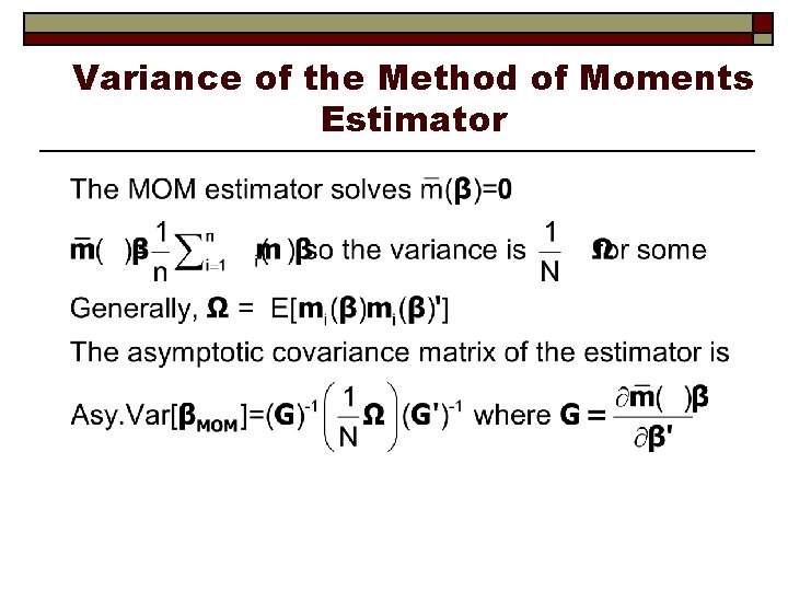
Variance of the Method of Moments Estimator

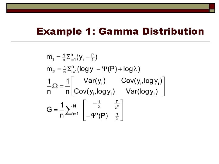
Example 1: Gamma Distribution

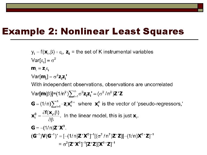
Example 2: Nonlinear Least Squares

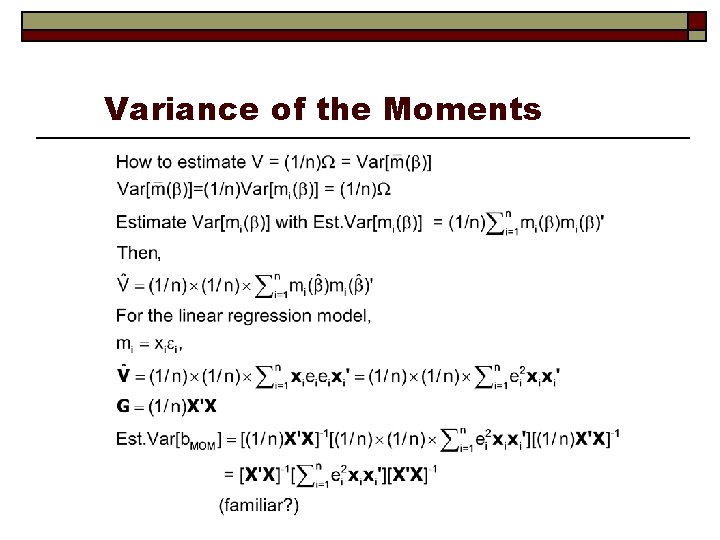
Variance of the Moments

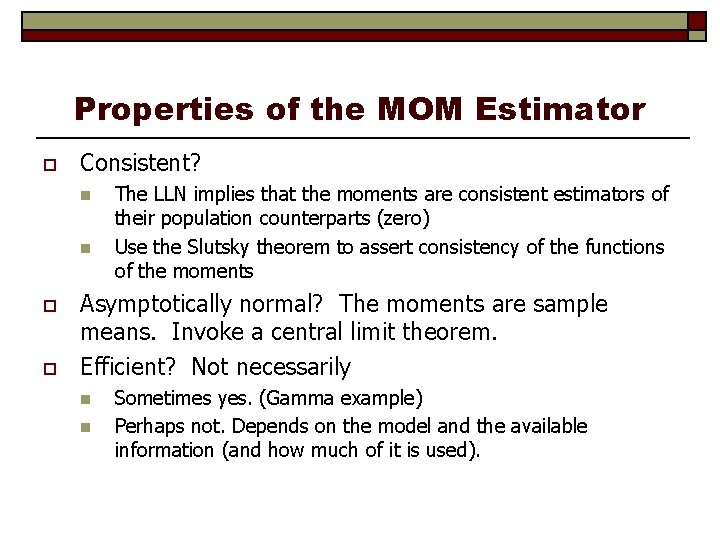
Properties of the MOM Estimator o Consistent? n n o o The LLN implies that the moments are consistent estimators of their population counterparts (zero) Use the Slutsky theorem to assert consistency of the functions of the moments Asymptotically normal? The moments are sample means. Invoke a central limit theorem. Efficient? Not necessarily n n Sometimes yes. (Gamma example) Perhaps not. Depends on the model and the available information (and how much of it is used).

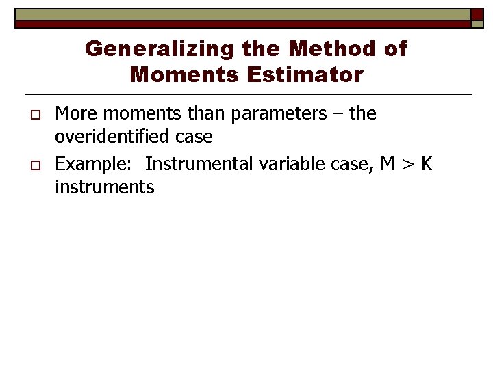
Generalizing the Method of Moments Estimator o o More moments than parameters – the overidentified case Example: Instrumental variable case, M > K instruments

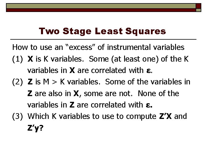
Two Stage Least Squares How to use an “excess” of instrumental variables (1) X is K variables. Some (at least one) of the K variables in X are correlated with ε. (2) Z is M > K variables. Some of the variables in Z are also in X, some are not. None of the variables in Z are correlated with ε. (3) Which K variables to use to compute Z’X and Z’y?

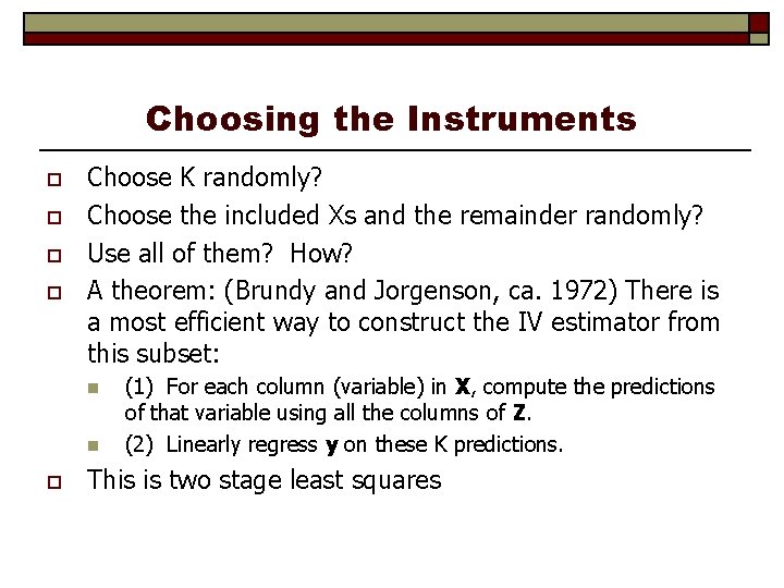
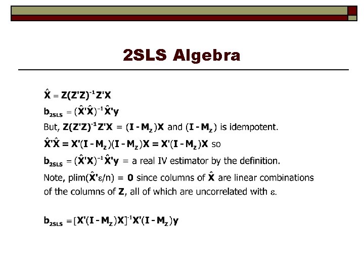
Choosing the Instruments o o Choose K randomly? Choose the included Xs and the remainder randomly? Use all of them? How? A theorem: (Brundy and Jorgenson, ca. 1972) There is a most efficient way to construct the IV estimator from this subset: n n o (1) For each column (variable) in X, compute the predictions of that variable using all the columns of Z. (2) Linearly regress y on these K predictions. This is two stage least squares

2 SLS Algebra

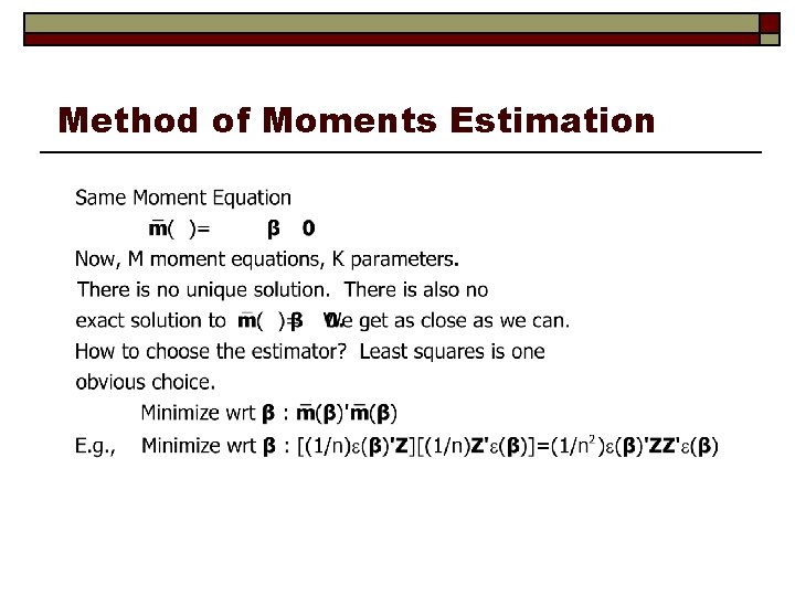
Method of Moments Estimation

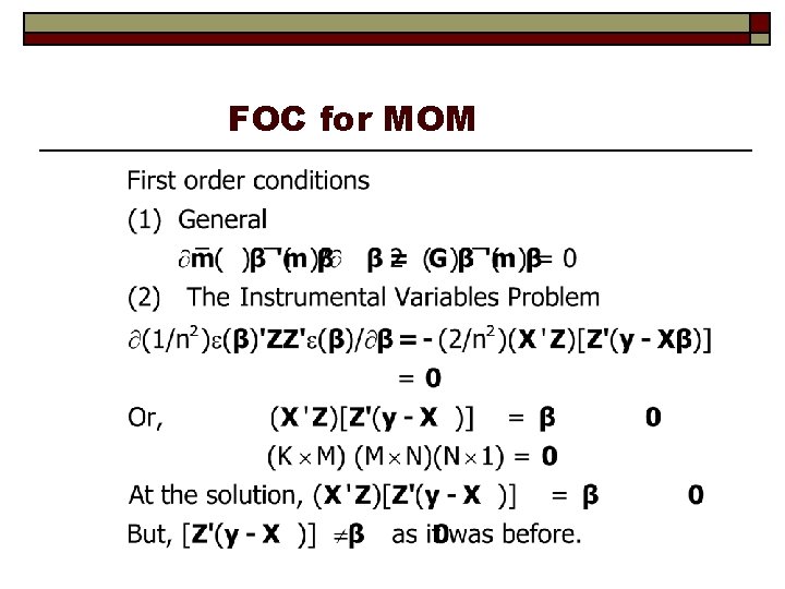
FOC for MOM

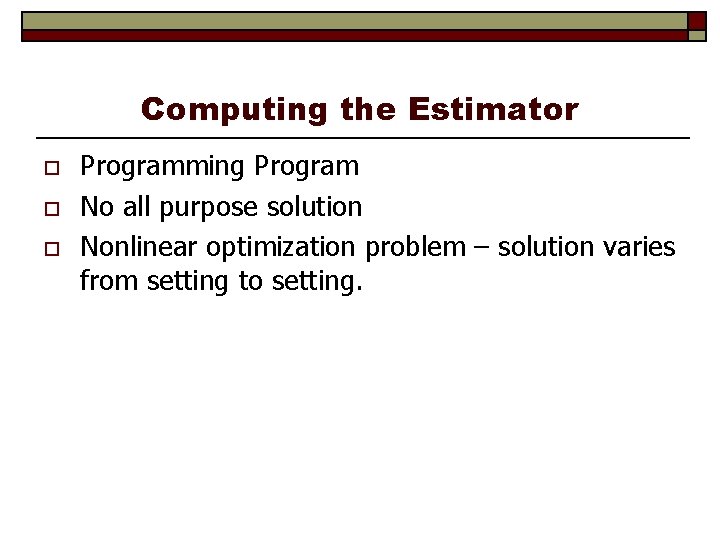
Computing the Estimator o o o Programming Program No all purpose solution Nonlinear optimization problem – solution varies from setting to setting.

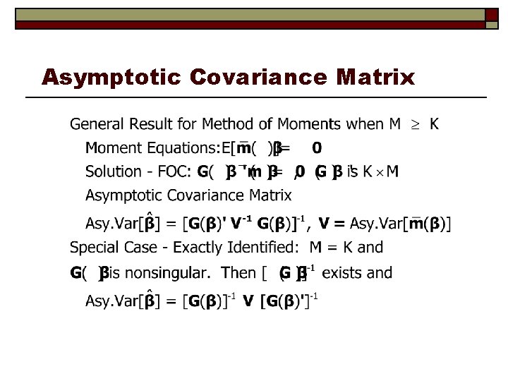
Asymptotic Covariance Matrix

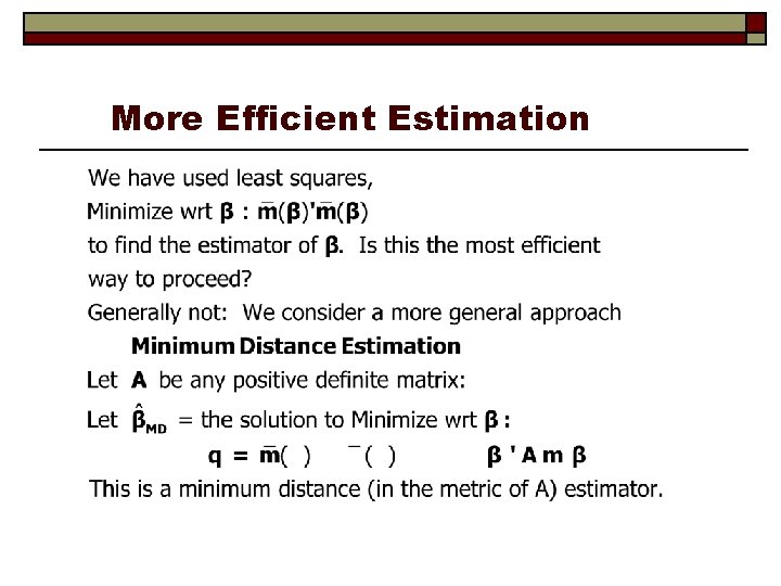
More Efficient Estimation

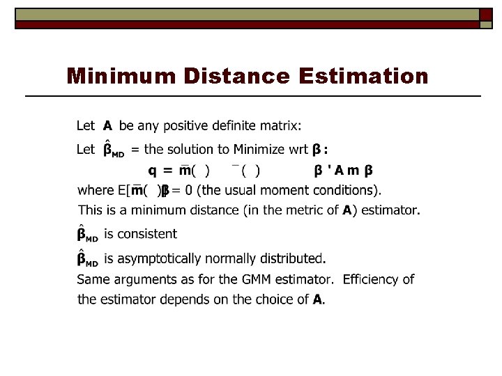
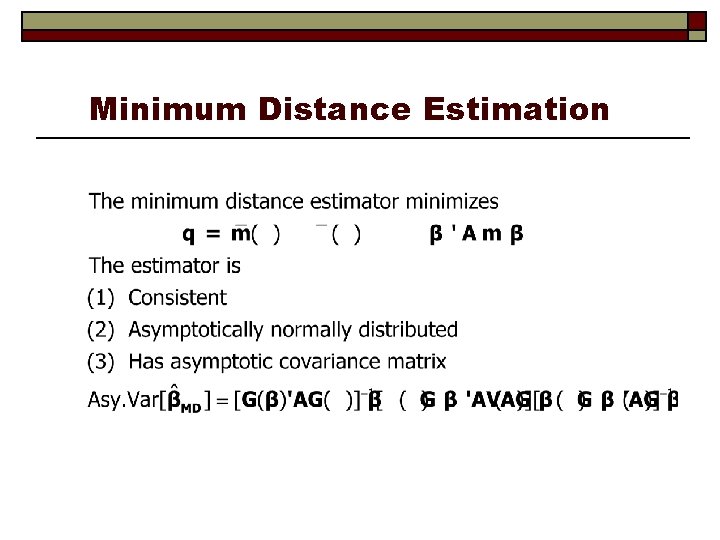
Minimum Distance Estimation

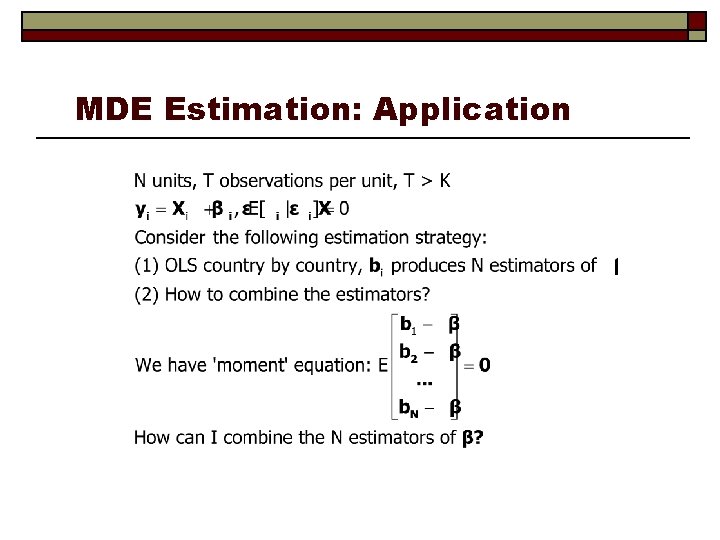
MDE Estimation: Application

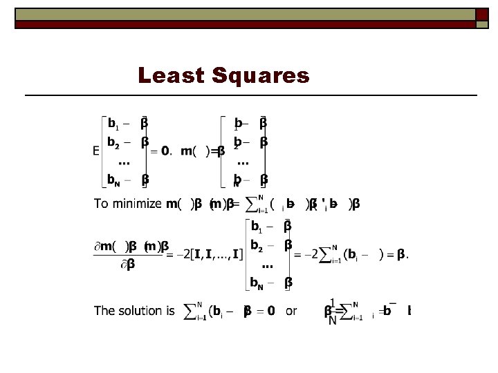
Least Squares

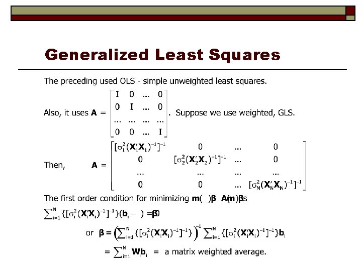
Generalized Least Squares

Minimum Distance Estimation

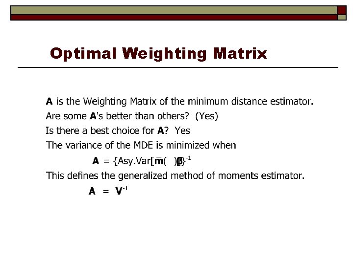
Optimal Weighting Matrix

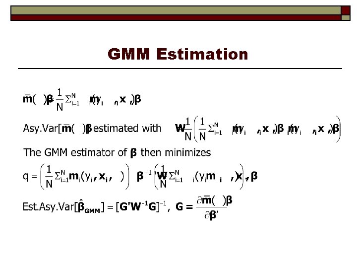
GMM Estimation

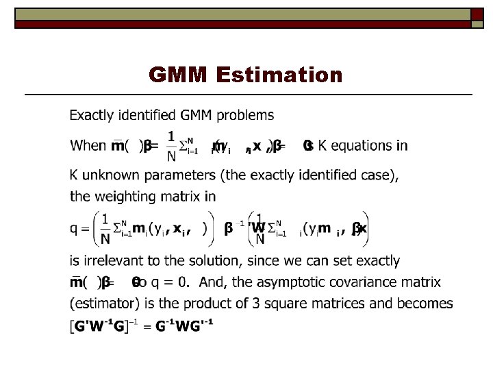
GMM Estimation

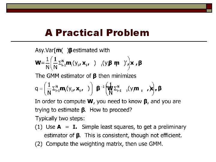
A Practical Problem

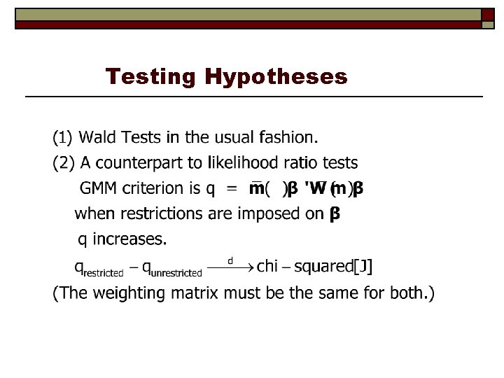
Testing Hypotheses

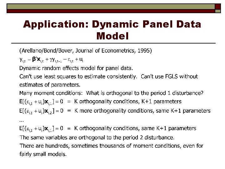
Application: Dynamic Panel Data Model