Econometrics Chengyuan Yin School of Mathematics Econometrics 24

Econometrics Chengyuan Yin School of Mathematics

Econometrics 24. Simulation Based Estimation

Settings o Conditional and unconditional log likelihoods n n o Bayesian estimation n n o Likelihood function to be maximized contains unobservables Integration techniques Prior times likelihood is intractible How to obtain posterior means, which are open form integrals The problem in both cases is “…how to do the integration? ”

A Conditional Log Likelihood

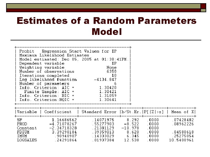
Application - Innovation o o Sample = 1, 270 German Manufacturing Firms Panel, 5 years, 1984 -1988 Response: Process or product innovation in the survey year? (yes or no) Inputs: n n n o o Imports of products in the industry Pressure from foreign direct investment Other covariates Model: Probit with common firm effects (Irene Bertschuk, doctoral thesis, Journal of Econometrics, 1998)

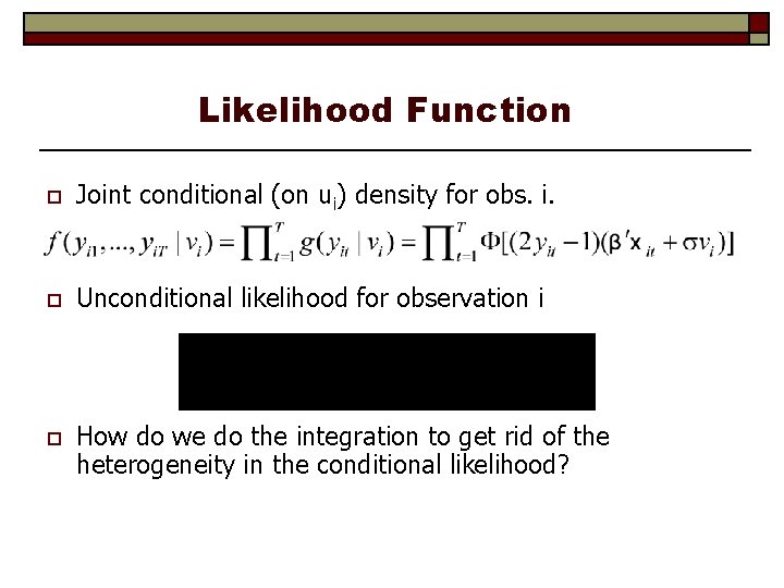
Likelihood Function o Joint conditional (on ui) density for obs. i. o Unconditional likelihood for observation i o How do we do the integration to get rid of the heterogeneity in the conditional likelihood?

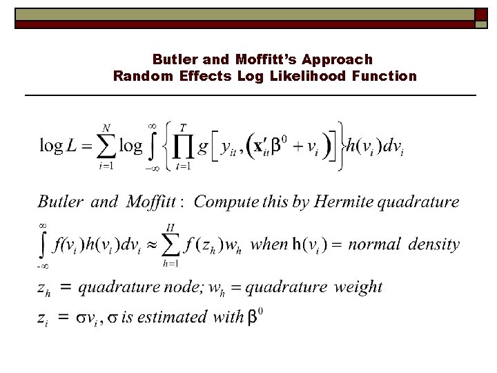
Obtaining the Unconditional Likelihood o The Butler and Moffitt (1982) method is used by most current software n n Quadrature Works for normally distributed heterogeneity

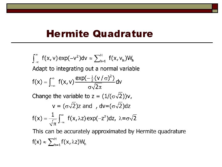
Hermite Quadrature

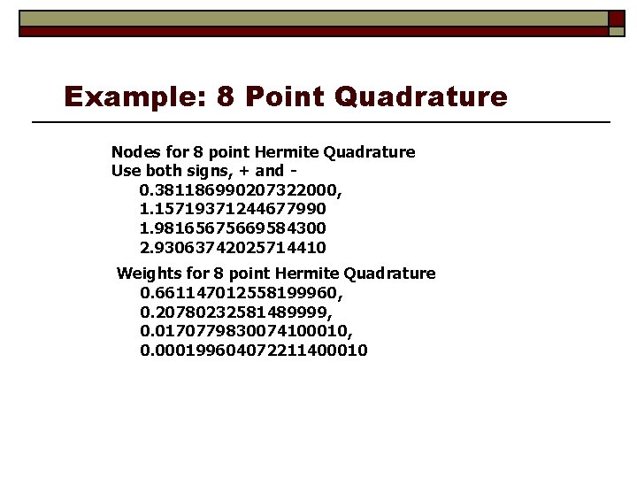
Example: 8 Point Quadrature Nodes for 8 point Hermite Quadrature Use both signs, + and 0. 381186990207322000, 1. 15719371244677990 1. 98165675669584300 2. 93063742025714410 Weights for 8 point Hermite Quadrature 0. 661147012558199960, 0. 20780232581489999, 0. 0170779830074100010, 0. 000199604072211400010

Butler and Moffitt’s Approach Random Effects Log Likelihood Function

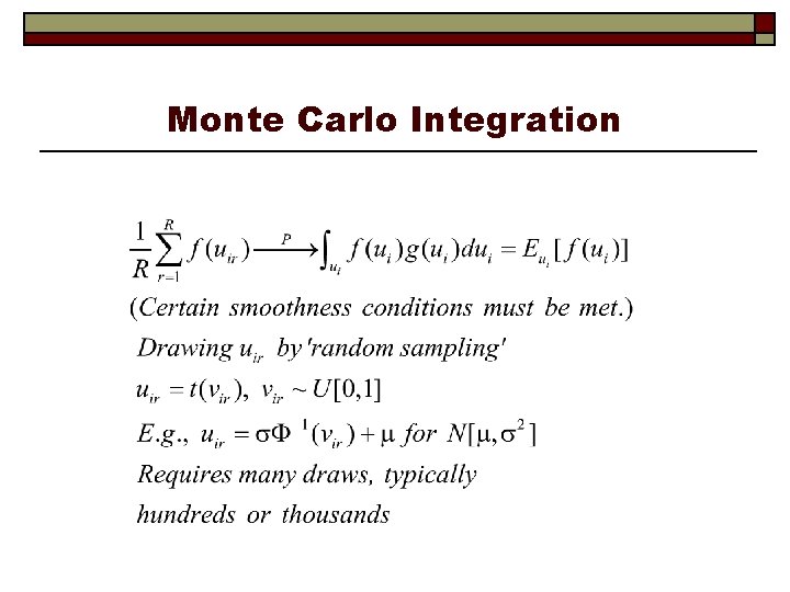
Monte Carlo Integration

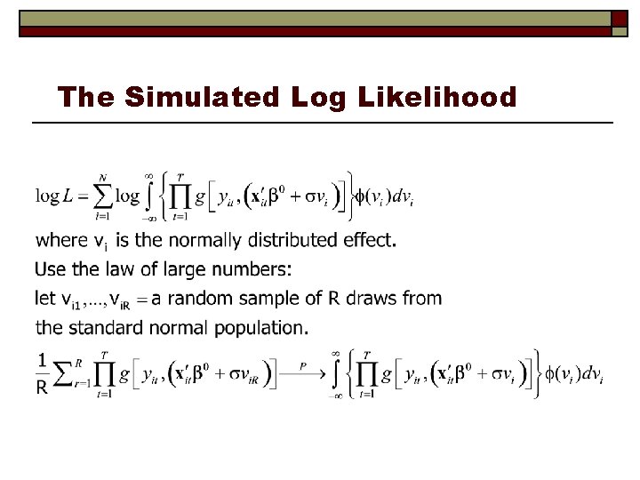
The Simulated Log Likelihood

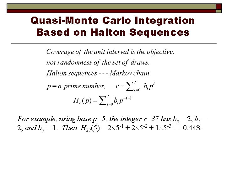
Quasi-Monte Carlo Integration Based on Halton Sequences For example, using base p=5, the integer r=37 has b 0 = 2, b 1 = 2, and b 3 = 1. Then H 37(5) = 2 5 -1 + 2 5 -2 + 1 5 -3 = 0. 448.

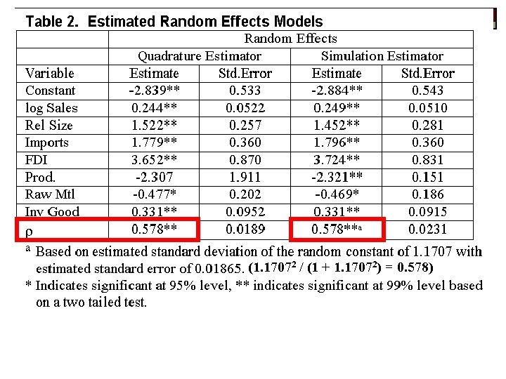
Panel Data Estimation A Random Effects Probit Model

Log Likelihood

(1. 17072 / (1 + 1. 17072) = 0. 578)

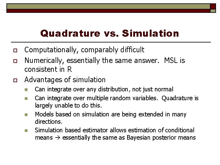
Quadrature vs. Simulation o o o Computationally, comparably difficult Numerically, essentially the same answer. MSL is consistent in R Advantages of simulation n n Can integrate over any distribution, not just normal Can integrate over multiple random variables. Quadrature is largely unable to do this. Models based on simulation are being extended in many directions. Simulation based estimator allows estimation of conditional means essentially the same as Bayesian posterior means

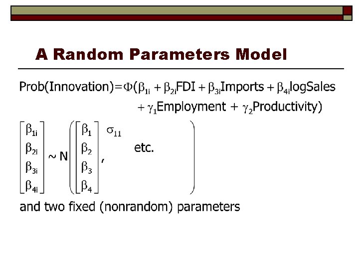
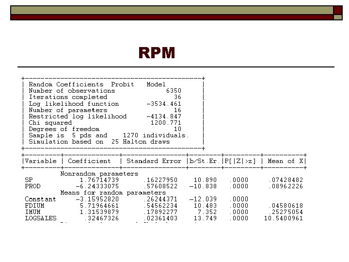
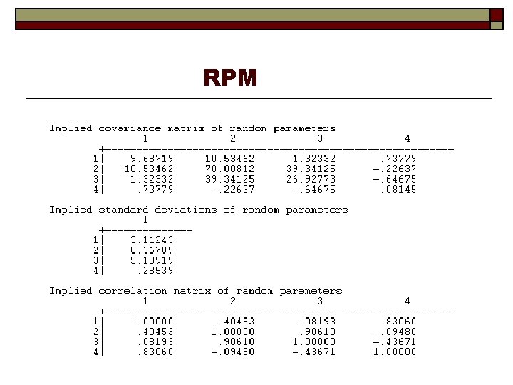
A Random Parameters Model

Estimates of a Random Parameters Model

RPM

RPM

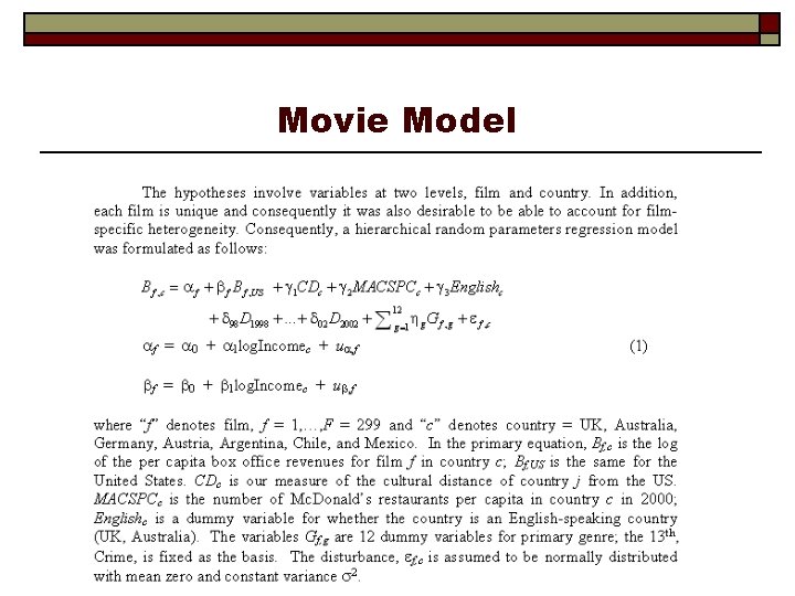
Movie Model

Parameter Heterogeneity

Bayesian Estimators o o “Random Parameters” Models of Individual Heterogeneity n n Random Effects: Consumer Brand Choice Fixed Effects: Hospital Costs

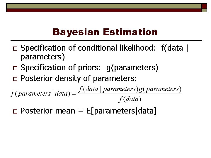
Bayesian Estimation o Specification of conditional likelihood: f(data | parameters) Specification of priors: g(parameters) Posterior density of parameters: o Posterior mean = E[parameters|data] o o

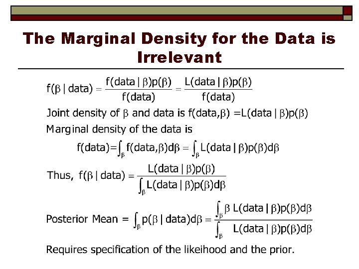
The Marginal Density for the Data is Irrelevant

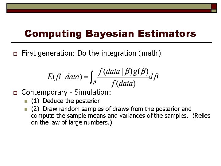
Computing Bayesian Estimators o First generation: Do the integration (math) o Contemporary - Simulation: n n (1) Deduce the posterior (2) Draw random samples of draws from the posterior and compute the sample means and variances of the samples. (Relies on the law of large numbers. )

Modeling Issues o o As N , the likelihood dominates and the prior disappears Bayesian and Classical MLE converge. (Needs the mode of the posterior to converge to the mean. ) Priors n n Diffuse large variances imply little prior information. (NONINFORMATIVE) INFORMATIVE priors – finite variances that appear in the posterior. “Taints” any final results.

A Random Effects Approach o Allenby and Rossi, “Marketing Models of Consumer Heterogeneity” n n n o Discrete Choice Model – Brand Choice “Hierarchical Bayes” Multinomial Probit Panel Data: Purchases of 4 brands of Ketchup

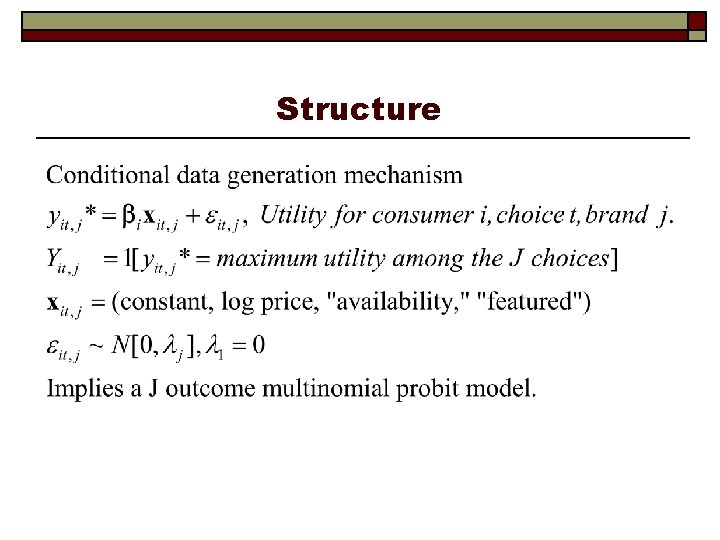
Structure

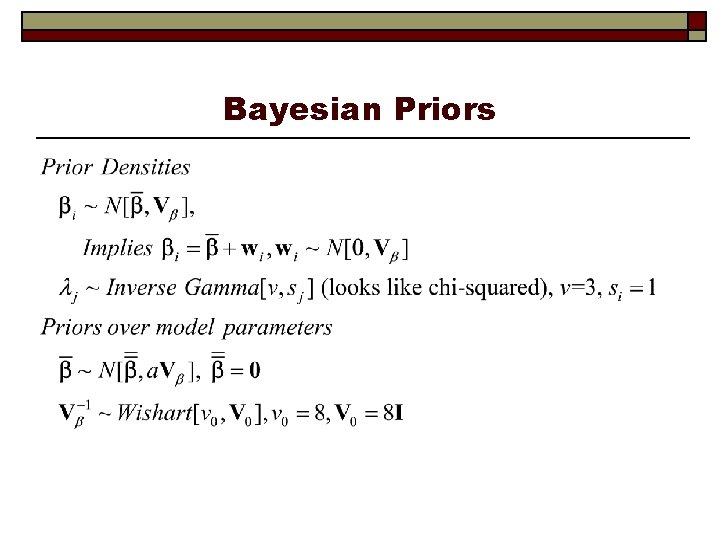
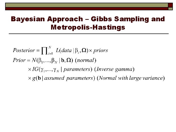
Bayesian Priors

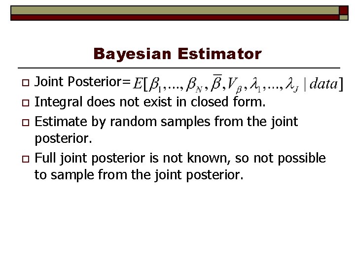
Bayesian Estimator o o Joint Posterior= Integral does not exist in closed form. Estimate by random samples from the joint posterior. Full joint posterior is not known, so not possible to sample from the joint posterior.

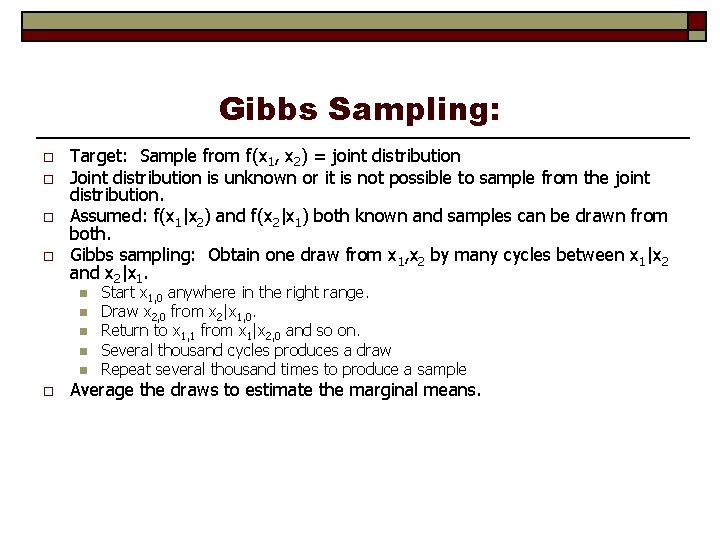
Gibbs Sampling: o o Target: Sample from f(x 1, x 2) = joint distribution Joint distribution is unknown or it is not possible to sample from the joint distribution. Assumed: f(x 1|x 2) and f(x 2|x 1) both known and samples can be drawn from both. Gibbs sampling: Obtain one draw from x 1, x 2 by many cycles between x 1|x 2 and x 2|x 1. n n n o Start x 1, 0 anywhere in the right range. Draw x 2, 0 from x 2|x 1, 0. Return to x 1, 1 from x 1|x 2, 0 and so on. Several thousand cycles produces a draw Repeat several thousand times to produce a sample Average the draws to estimate the marginal means.

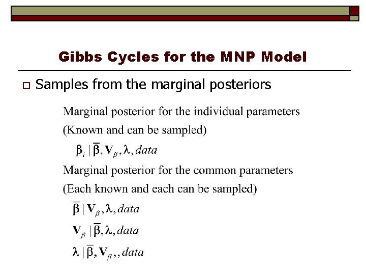
Gibbs Cycles for the MNP Model o Samples from the marginal posteriors

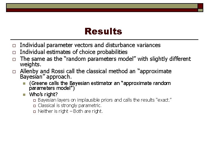
Results o o Individual parameter vectors and disturbance variances Individual estimates of choice probabilities The same as the “random parameters model” with slightly different weights. Allenby and Rossi call the classical method an “approximate Bayesian” approach. n n (Greene calls the Bayesian estimator an “approximate random parameters model”) Who’s right? o o o Bayesian layers on implausible priors and calls the results “exact. ” Classical is strongly parametric. Neither is right – Both are right.

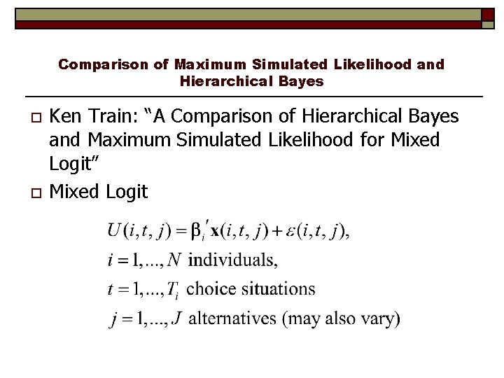
Comparison of Maximum Simulated Likelihood and Hierarchical Bayes o o Ken Train: “A Comparison of Hierarchical Bayes and Maximum Simulated Likelihood for Mixed Logit” Mixed Logit

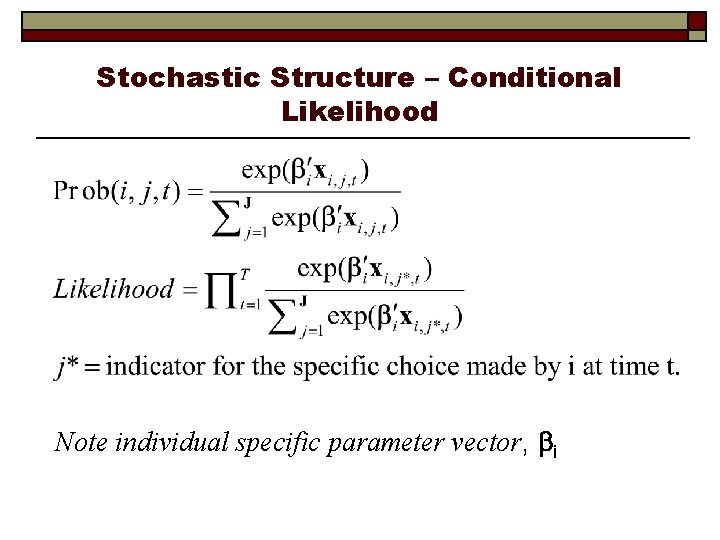
Stochastic Structure – Conditional Likelihood Note individual specific parameter vector, i

Classical Approach

Bayesian Approach – Gibbs Sampling and Metropolis-Hastings

Gibbs Sampling from Posteriors: b

Gibbs Sampling from Posteriors: Ω

Gibbs Sampling from Posteriors: i

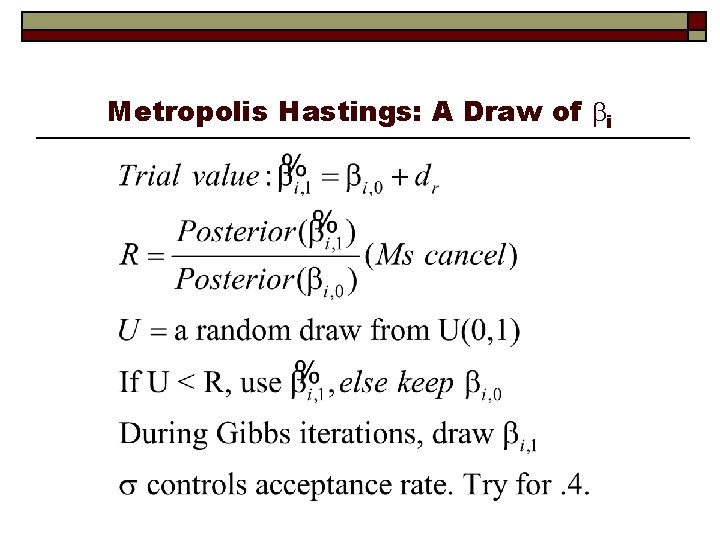
Metropolis – Hastings Method

Metropolis Hastings: A Draw of i

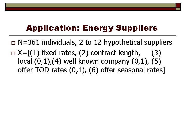
Application: Energy Suppliers o o N=361 individuals, 2 to 12 hypothetical suppliers X=[(1) fixed rates, (2) contract length, (3) local (0, 1), (4) well known company (0, 1), (5) offer TOD rates (0, 1), (6) offer seasonal rates]

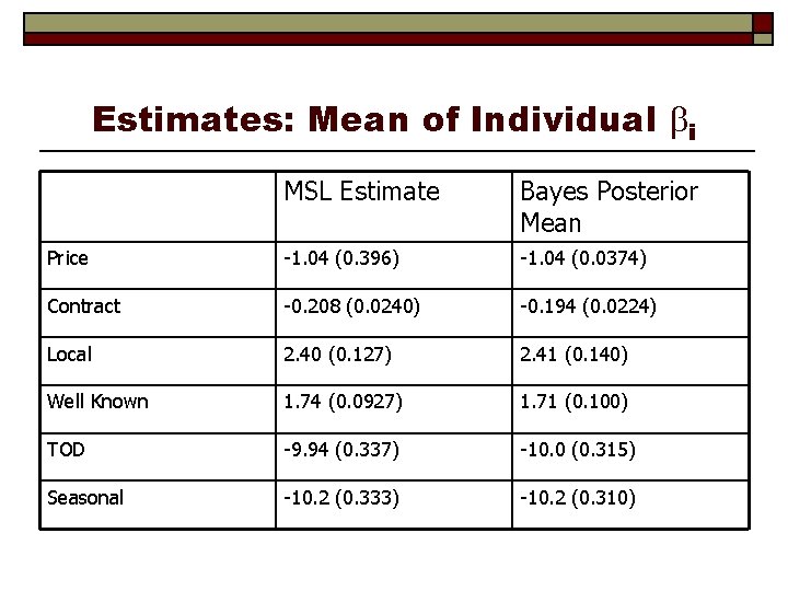
Estimates: Mean of Individual i MSL Estimate Bayes Posterior Mean Price -1. 04 (0. 396) -1. 04 (0. 0374) Contract -0. 208 (0. 0240) -0. 194 (0. 0224) Local 2. 40 (0. 127) 2. 41 (0. 140) Well Known 1. 74 (0. 0927) 1. 71 (0. 100) TOD -9. 94 (0. 337) -10. 0 (0. 315) Seasonal -10. 2 (0. 333) -10. 2 (0. 310)

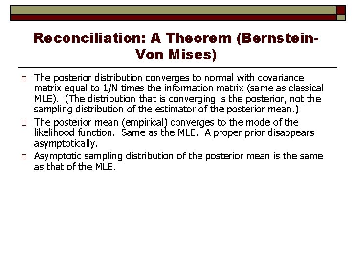
Reconciliation: A Theorem (Bernstein. Von Mises) o o o The posterior distribution converges to normal with covariance matrix equal to 1/N times the information matrix (same as classical MLE). (The distribution that is converging is the posterior, not the sampling distribution of the estimator of the posterior mean. ) The posterior mean (empirical) converges to the mode of the likelihood function. Same as the MLE. A proper prior disappears asymptotically. Asymptotic sampling distribution of the posterior mean is the same as that of the MLE.