CSE 3813 Introduction to Formal Languages and Automata

CSE 3813 Introduction to Formal Languages and Automata Chapter 9 The Standard Turing Machine These class notes are based on material from our textbook, An Introduction to Formal Languages and Automata, 4 th ed. , by Peter Linz, published by Jones and Bartlett Publishers, Inc. , Sudbury, MA, 2006. They are intended for classroom use only and are not a substitute for reading the textbook.

Diagrams from some slides are from previous year’s textbook: Martin, John C. , Introduction to Languages and the Theory of Computation. Boston: WCG Mc. Graw. Hill, 1991. Slides are for use of this class only.

Automata A Finite Automaton has only its states to serve as memory - very limited in what languages it could recognize In a Pushdown Automaton we added a stack to a Finite Automaton - this gave it better memory, and allowed it to recognize more languages. But it was still limited by the nature of the stack. We could add another stack to a Pushdown Automaton. This would allow it to accept some non-context free languages (e. g. , anbncn). Or we could change the stack to a queue. This would allow other languages to be accepted (e. g. , ww).

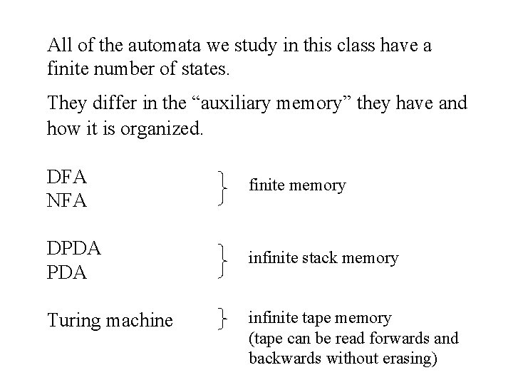
All of the automata we study in this class have a finite number of states. They differ in the “auxiliary memory” they have and how it is organized. DFA NFA finite memory DPDA infinite stack memory Turing machine infinite tape memory (tape can be read forwards and backwards without erasing)

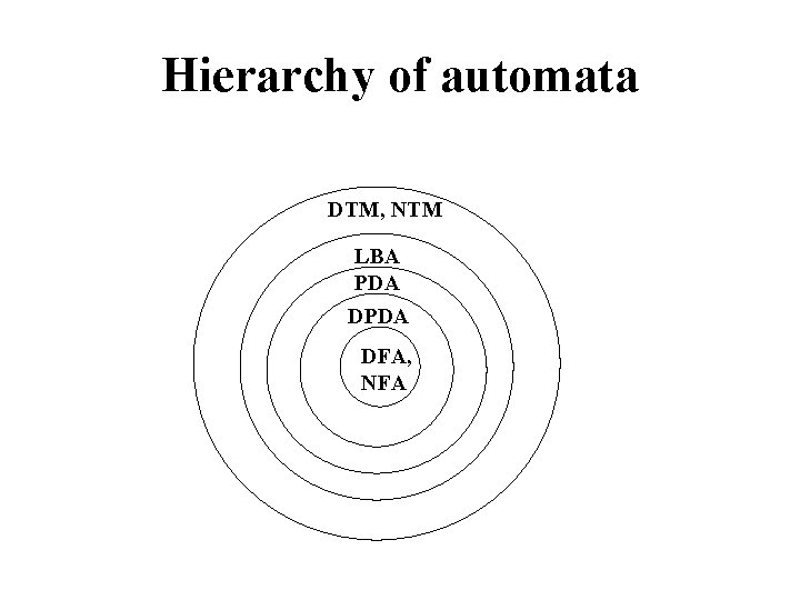
Hierarchy of automata DTM, NTM LBA PDA DFA, NFA

The Turing Machine Alan Mathison Turing, b. 1912, d. 1954. Contributed much to the foundations of computing theory. Published the Turing machine model in 1937. Church-Turing Thesis - “Any algorithmic procedure that can be carried out by a human, a team of humans, or a machine can be carried out by some Turing machine. ” Unproveable, because we don’t have a precise definition of what “algorithmic procedure” means, but generally accepted as true. Puts a limit on what can be computed.

The Church-Turing Thesis • No model of digital computation is more powerful than a Turing machine. • By “more powerful, ” we mean “can recognize languages that a TM cannot recognize. ” • This is not something that can be proved. But everybody believes it because no one has been able to devise a more powerful model of computation.

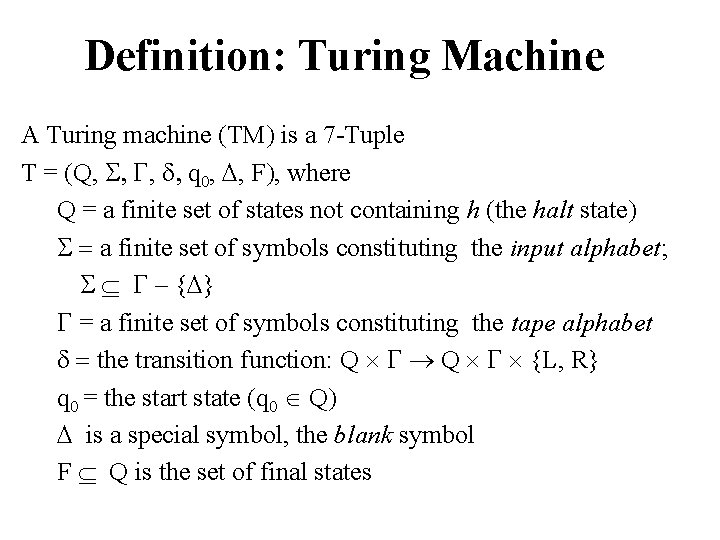
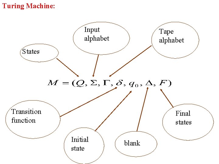
Definition: Turing Machine A Turing machine (TM) is a 7 -Tuple T = (Q, S, , , q 0, , F), where Q = a finite set of states not containing h (the halt state) S = a finite set of symbols constituting the input alphabet; S – { } = a finite set of symbols constituting the tape alphabet = the transition function: Q Q {L, R} q 0 = the start state (q 0 Q) is a special symbol, the blank symbol F Q is the set of final states

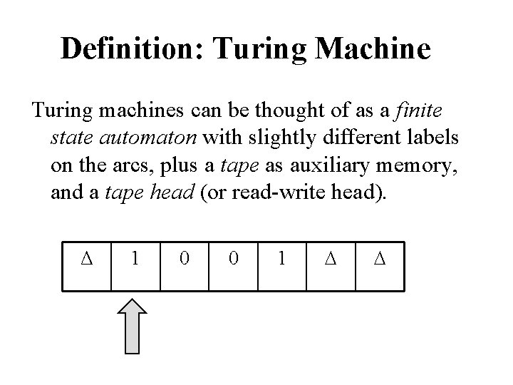
Definition: Turing Machine Turing machines can be thought of as a finite state automaton with slightly different labels on the arcs, plus a tape as auxiliary memory, and a tape head (or read-write head). Δ 1 0 0 1

Definition: Turing Machine The tape on a Turing machine can be thought of as a linear structure marked off into squares or cells. It is usually defined as infinite in both directions, but may be thought of as bounded on the left side, but infinite on the right.

Definition: Turing Machine Each cell on the tape on a Turing machine can hold: • a symbol from the input alphabet, or • a symbol from the tape alphabet (which may include some symbols which are not in the input alphabet), or • a blank symbol , which is distinct from the input alphabet.

Standard Turing Machine The standard Turing machine described by our textbook has several features: The TM has a tape that is unbounded in both directions. The TM is deterministic in the sense that defines at most one move per configuration There is no special input file; the input is copied onto the tape. There is no special output device; the tape contains the output, if any.

The TM tape head • The Turing machine has a tape head which reads from and writes to the tape during each move. • The tape head can move right or left, or may stay in the same position. • The tape head can read a character from the cell under which it is positioned, or it may write a character to the cell.

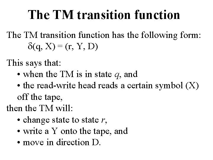
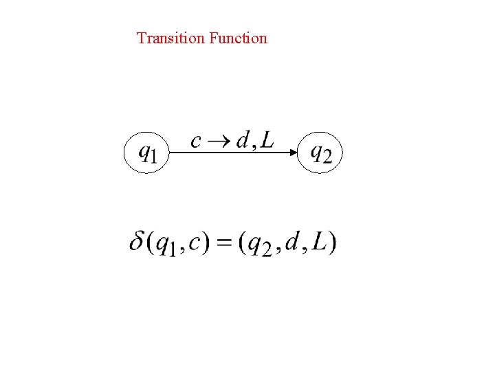
The TM transition function has the following form: (q, X) = (r, Y, D) This says that: • when the TM is in state q, and • the read-write head reads a certain symbol (X) off the tape, then the TM will: • change state to state r, • write a Y onto the tape, and • move in direction D.

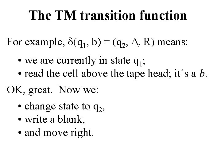
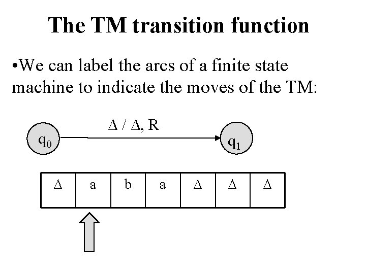
The TM transition function For example, (q 1, b) = (q 2, , R) means: • we are currently in state q 1; • read the cell above the tape head; it’s a b. OK, great. Now we: • change state to q 2, • write a blank, • and move right.

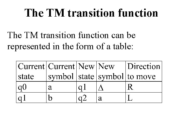
The TM transition function can be represented in the form of a table:

The TM transition function • We can label the arcs of a finite state machine to indicate the moves of the TM: / , R q 0 a b q 1 a

Processing a string • To process a string, we place the string onto the tape, where it can be read by the read-write head, surrounded by blank symbols on the left and right ends of the input. • Once the string is on the tape, then processing can begin. • We don’t need a separate input string after that.

Accepting a string There is only one way that a string may be accepted by a TM: • If a move causes the machine to move into an accepting halt state, then we stop and accept the string. (There are no moves out of a halt state. ) This may occur even when we haven’t finished processing the string yet.

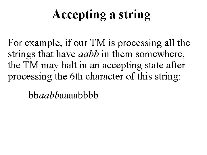
Accepting a string For example, if our TM is processing all the strings that have aabb in them somewhere, the TM may halt in an accepting state after processing the 6 th character of this string: bbaaaabbbb

Accepting a string If T = (Q, S, , , q 0, , F) is a Turing machine, and w S+, then w is accepted by T if, starting in the initial configuration corresponding to input w, T eventually enters a final acceptance state and halts.

Accepting a string In other words, w is accepted if there exists y and z * so that q 0 w |-T* yqfz, for some qf F In this situation, we say that T halts on input w. The language accepted by T is the set L(T) of input strings on which T halts.

Crashing and Halting There are 2 ways a string may fail to be accepted by a TM: • Crashing • Looping If the TM crashes, the string is explicitly rejected. If the TM loops forever, the string is implicitly rejected.

Crashing and Halting Crashing a. If a symbol is found on the tape for which the transition function is undefined, and the current state is not the accepting halt state, then we crash. b. If our TM has a bounded left end, and a move is specified which causes the machine to move off of the left end of the tape, then we crash.

Crashing and Halting Looping If an input string causes the TM to enter an infinite loop, then we loop forever.

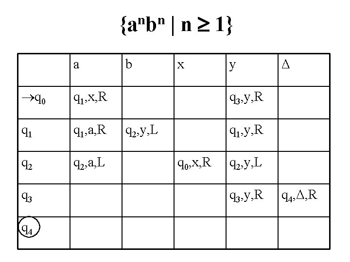
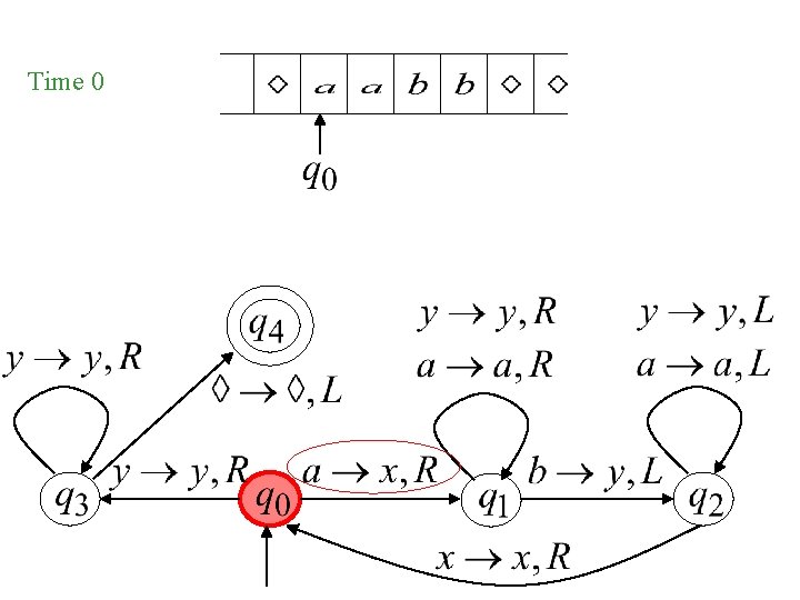
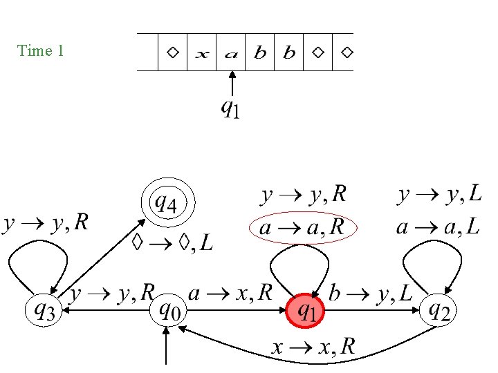
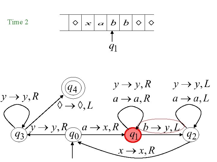
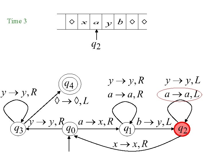
Exercises Design a TM that accepts L = {anbn | n 1} To do this, we can construct the transition table for the TM. We can use a matrix as a short-hand representation:

{anbn | n 1} a q 0 q 1, x, R q 1, a, R q 2, a, L q 3 q 4 b x y Δ q 3, y, R q 2, y, L q 1, y, R q 0, x, R q 2, y, L q 3, y, R q 4, Δ, R

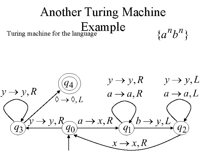
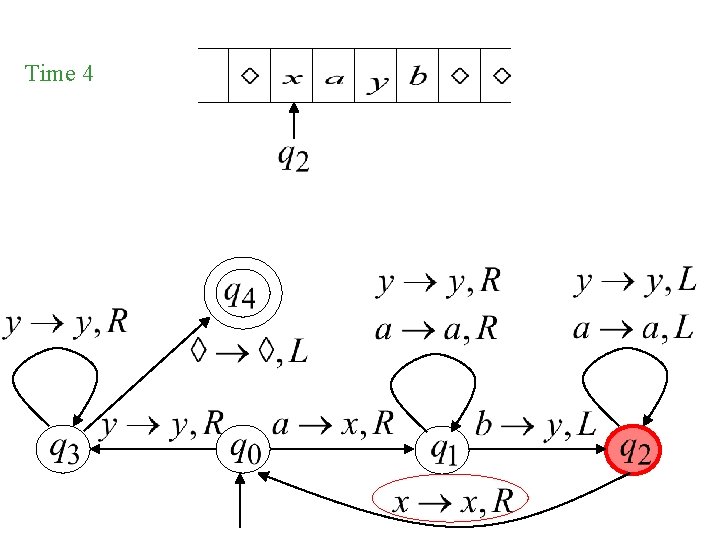
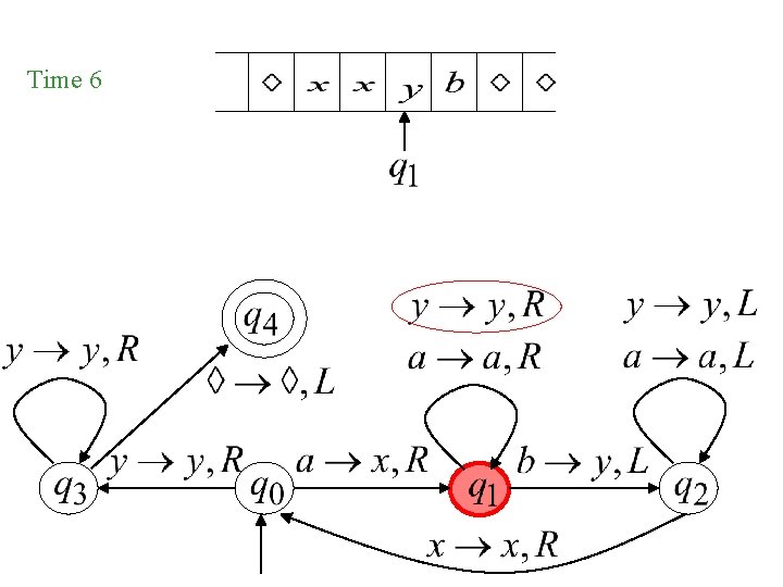
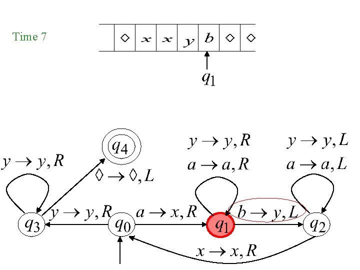
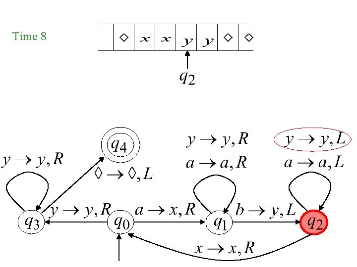
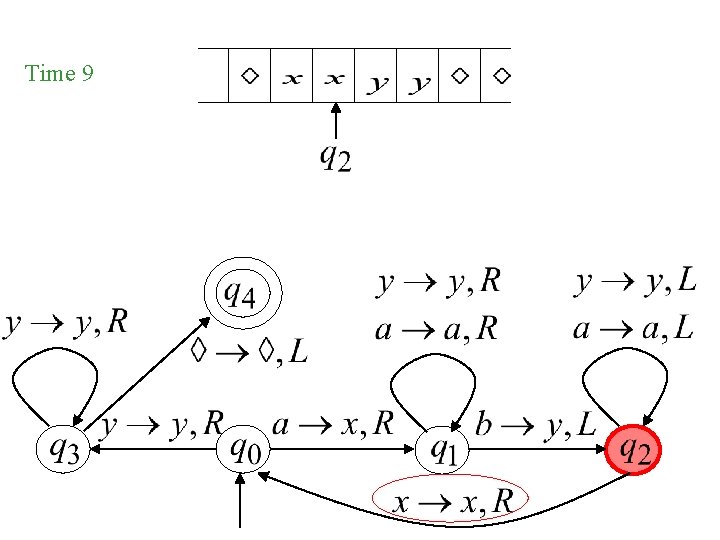
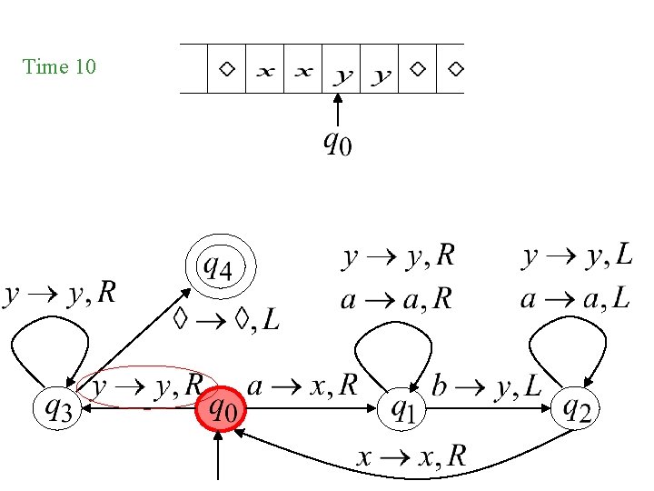
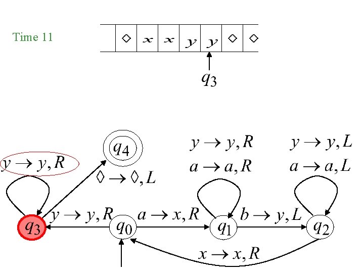
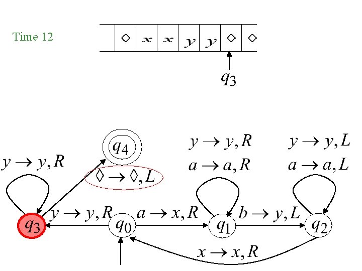
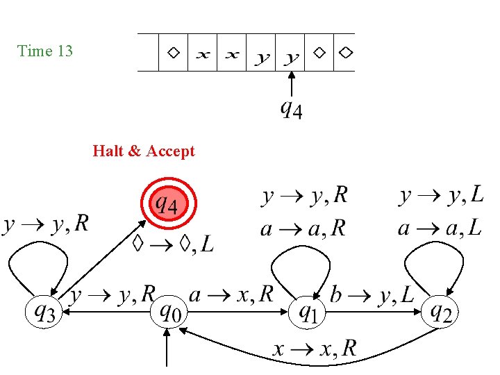
Another Turing Machine Example Turing machine for the language

Time 0

Time 1

Time 2

Time 3

Time 4

Time 5

Time 6

Time 7

Time 8

Time 9

Time 10

Time 11

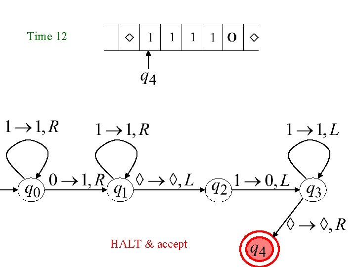
Time 12

Time 13 Halt & Accept

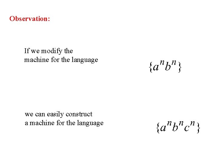
Observation: If we modify the machine for the language we can easily construct a machine for the language

Formal Definitions for Turing Machines

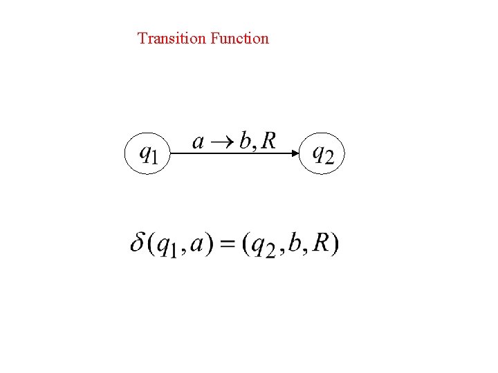
Transition Function

Transition Function

Turing Machine: Input alphabet Tape alphabet States Transition function Final states Initial state blank

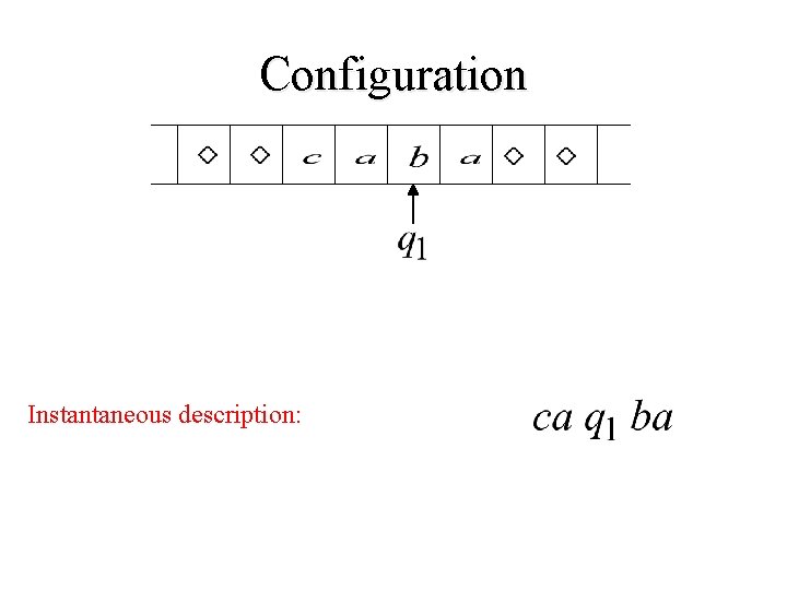
Configuration Instantaneous description:

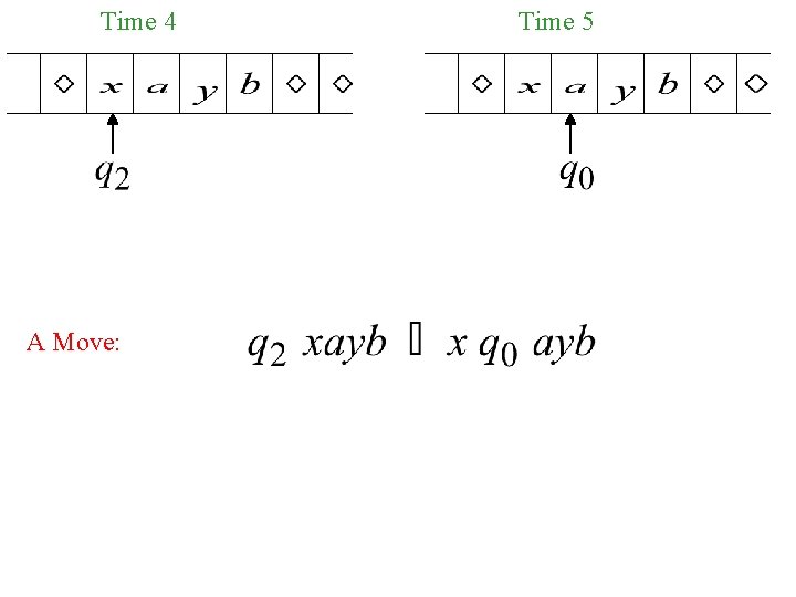
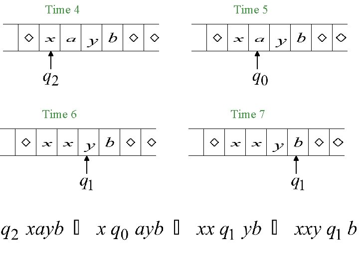
Time 4 A Move: Time 5

Time 4 Time 5 Time 6 Time 7

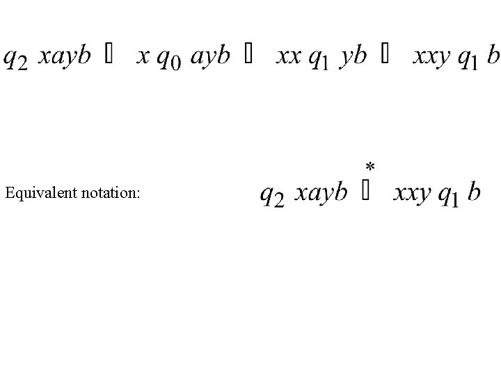
Equivalent notation:

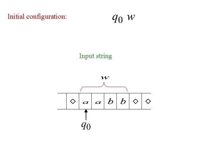
Initial configuration: Input string

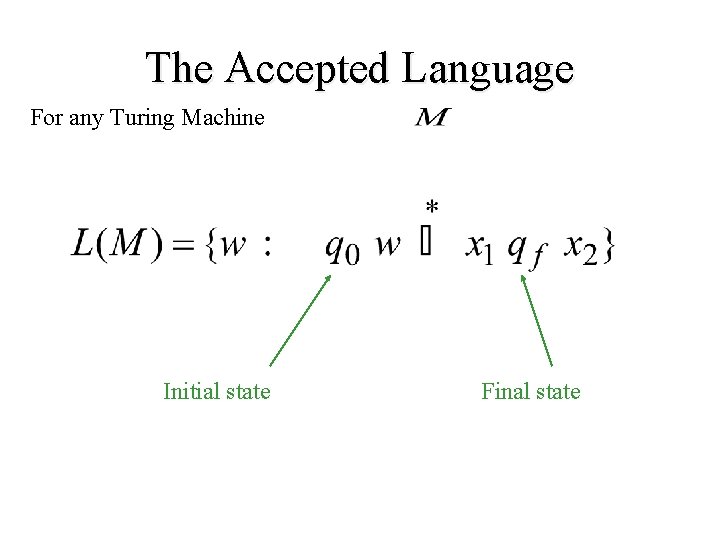
The Accepted Language For any Turing Machine Initial state Final state

Standard Turing Machine The machine we described is the standard: • Deterministic • Infinite tape in both directions • Tape is the input/output file

Computing Functions with Turing Machines

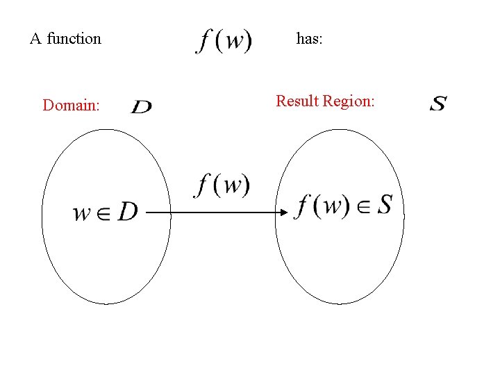
A function Domain: has: Result Region:

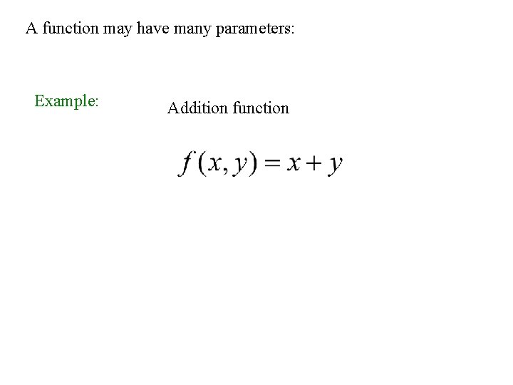
A function may have many parameters: Example: Addition function

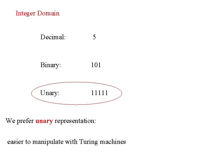
Integer Domain Decimal: 5 Binary: 101 Unary: 11111 We prefer unary representation: easier to manipulate with Turing machines

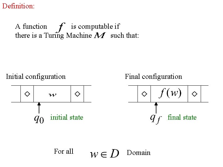
Definition: A function is computable if there is a Turing Machine such that: Initial configuration Final configuration initial state For all final state Domain

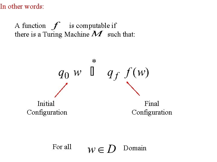
In other words: A function is computable if there is a Turing Machine such that: Initial Configuration For all Final Configuration Domain

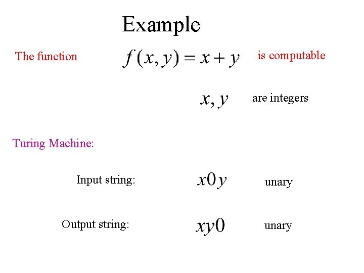
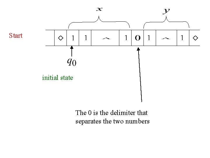
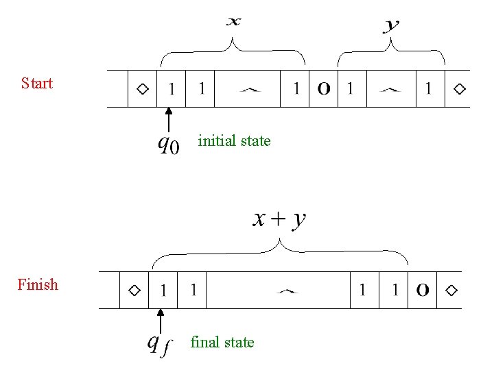
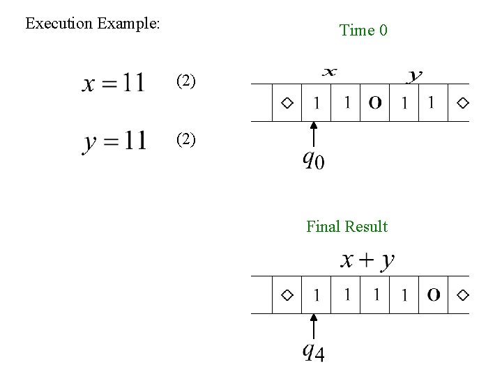
Example The function is computable are integers Turing Machine: Input string: Output string: unary

Start initial state The 0 is the delimiter that separates the two numbers

Start initial state Finish final state

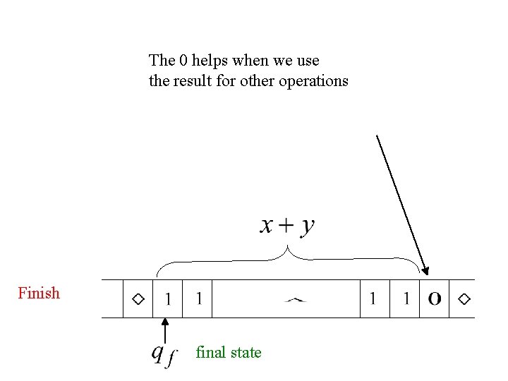
The 0 helps when we use the result for other operations Finish final state

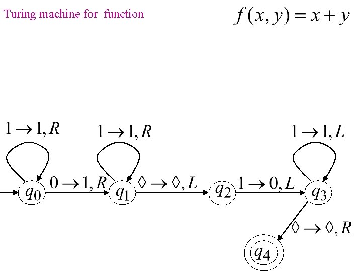
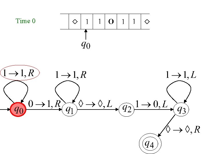
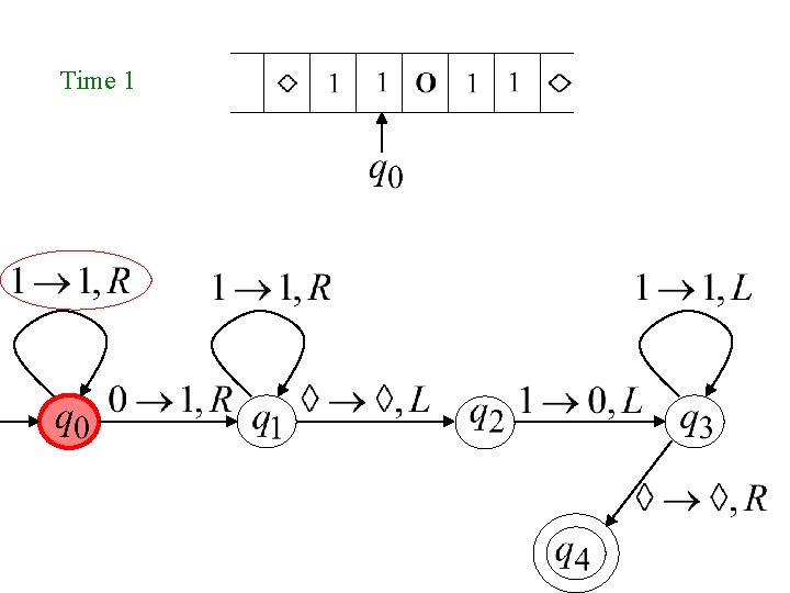
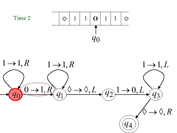
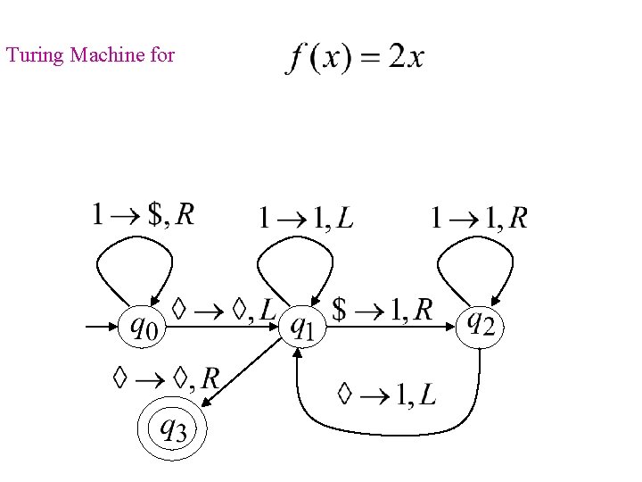
Turing machine for function

Execution Example: Time 0 (2) Final Result

Time 0

Time 1

Time 2

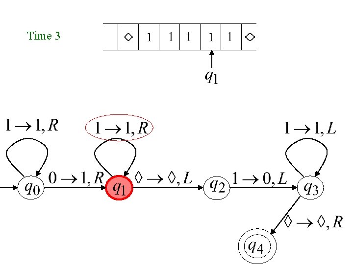
Time 3

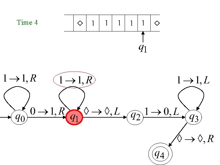
Time 4

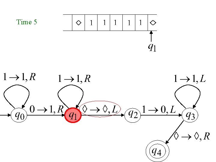
Time 5

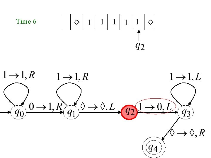
Time 6

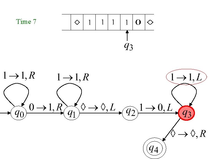
Time 7

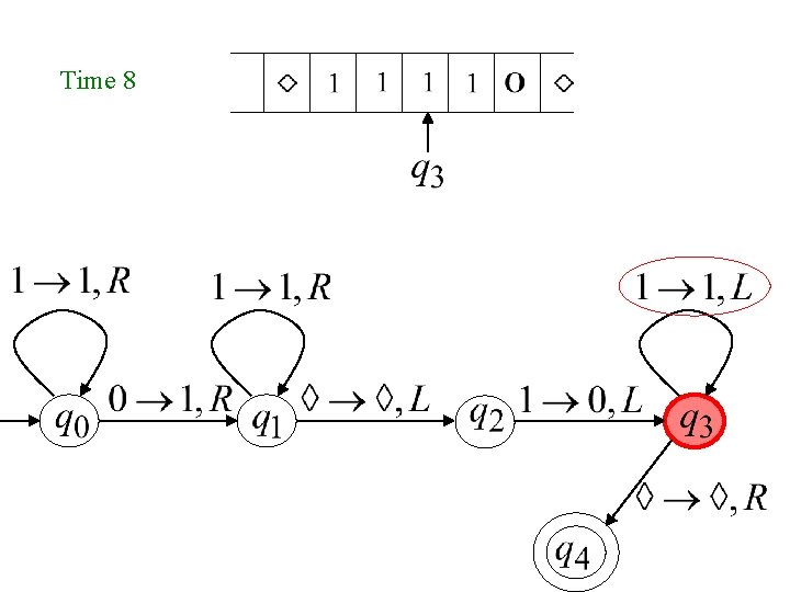
Time 8

Time 9

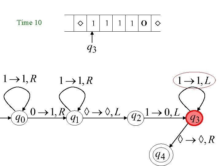
Time 10

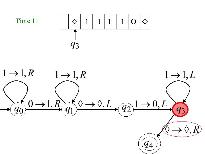
Time 11

Time 12 HALT & accept

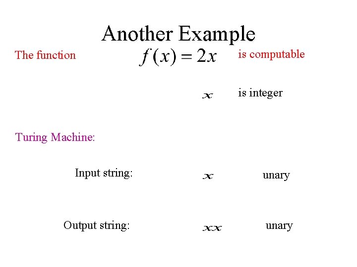
Another Example The function is computable is integer Turing Machine: Input string: unary Output string: unary

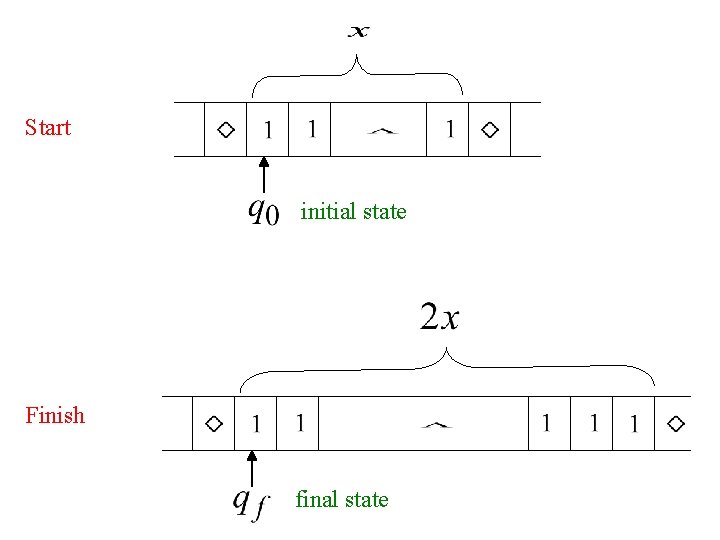
Start initial state Finish final state

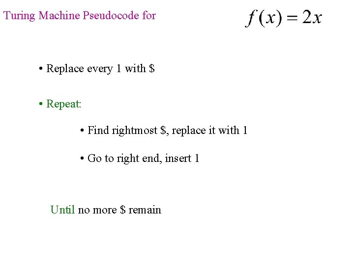
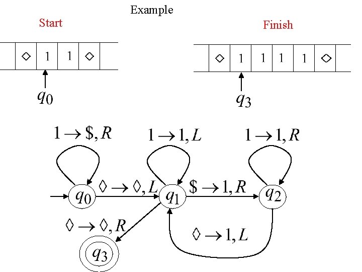
Turing Machine Pseudocode for • Replace every 1 with $ • Repeat: • Find rightmost $, replace it with 1 • Go to right end, insert 1 Until no more $ remain

Turing Machine for

Start Example Finish

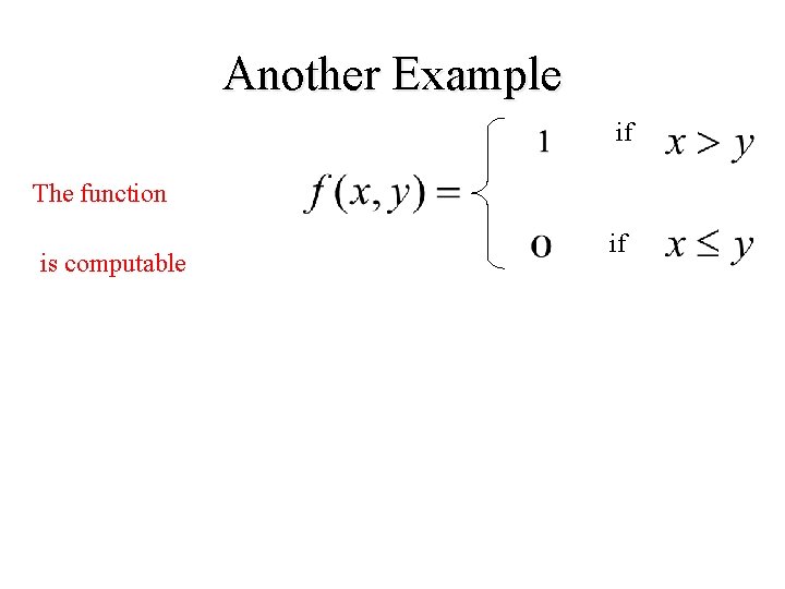
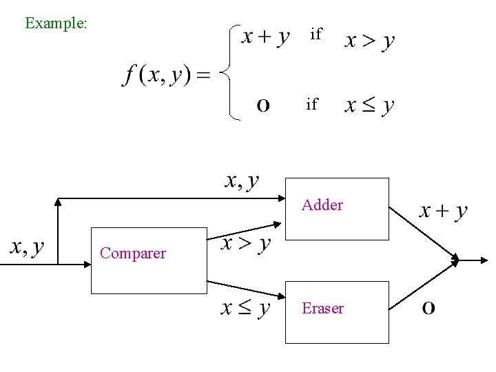
Another Example if The function is computable if

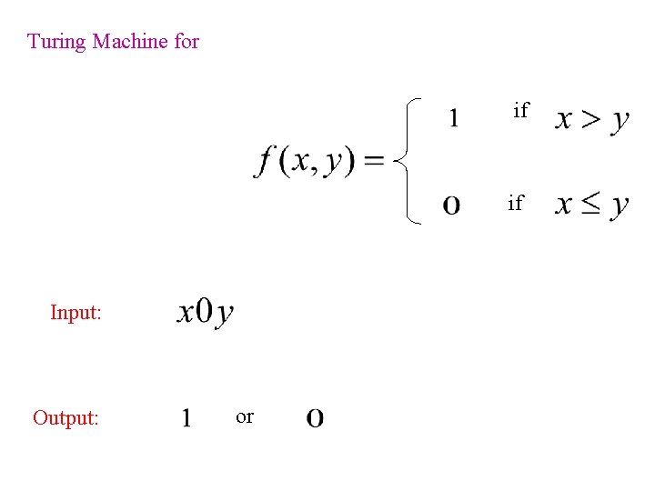
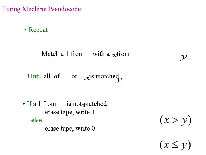
Turing Machine for if if Input: Output: or

Turing Machine Pseudocode: • Repeat Match a 1 from Until all of or with a 1 from is matched • If a 1 from is not matched erase tape, write 1 else erase tape, write 0

Combining Turing Machines

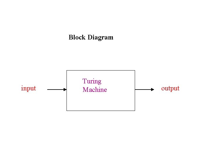
Block Diagram input Turing Machine output

Example: if if Adder Comparer Eraser

Exercises Work through the processing of the string w = aaabbb in class. Is this string accepted by the TM? Work through the processing of the string w = aaabb. Is this string accepted by the TM? How does the TM reject the string?

Exercises n Recall that the following languages are not context-free. – {anbncn | n 0} – {ww | w {a, b}*} n In English, describe how a Turing machine could accept each of these languages n Try to draw the transition diagrams for the Turing machines

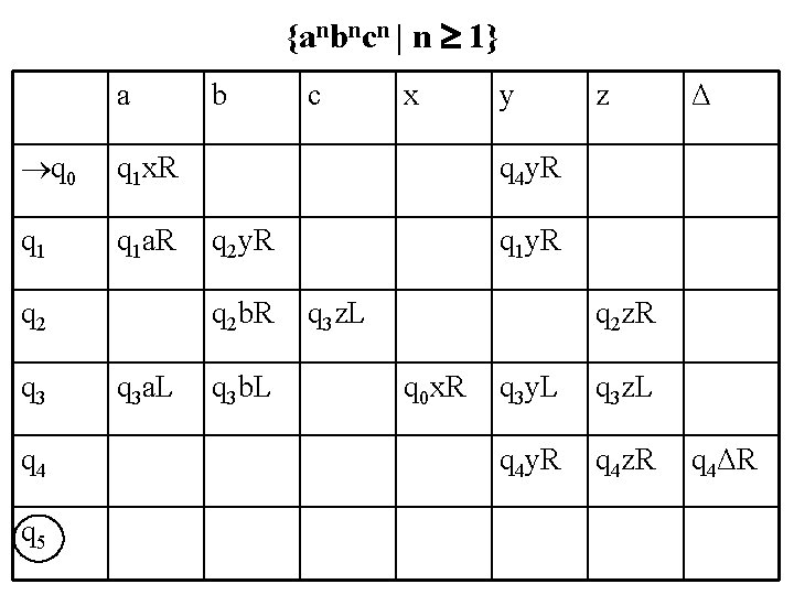
{anbncn | n 1} a q 0 q 1 x. R q 1 a. R q 2 q 3 q 4 q 5 b x y z Δ q 4 y. R q 2 b. R q 3 a. L c q 3 b. L q 1 y. R q 3 z. L q 2 z. R q 0 x. R q 3 y. L q 3 z. L q 4 y. R q 4 z. R q 4ΔR

Homework Suggestions n P. 236 -237 2, 3, 5, 7(a, b)

Model of computation n. A TM is an abstract model of a computer that lets us define in a precise, mathematical way what we mean by computation. n As before, we use the concept of a “configuration” to define what we mean by computation.

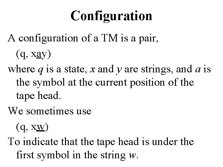
Configuration A configuration of a TM is a pair, (q, xay) where q is a state, x and y are strings, and a is the symbol at the current position of the tape head. We sometimes use (q, xw) To indicate that the tape head is under the first symbol in the string w.

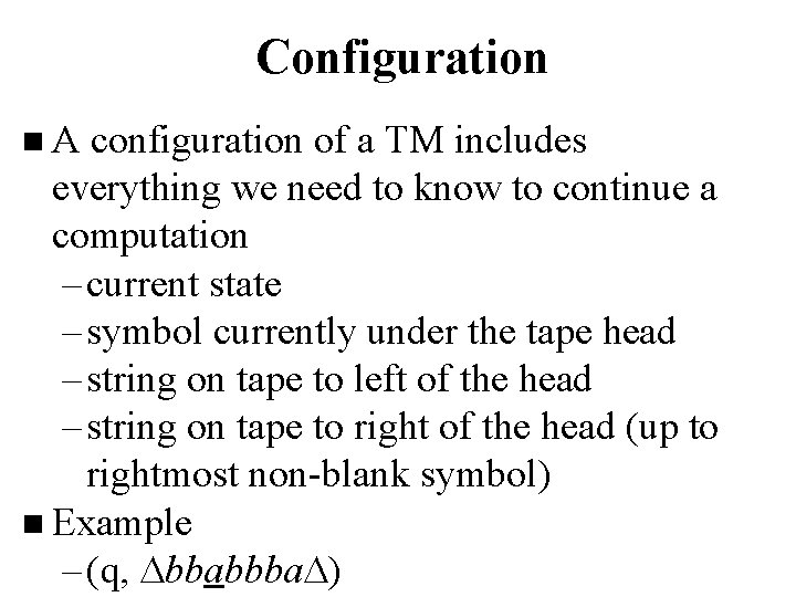
Configuration n. A configuration of a TM includes everything we need to know to continue a computation – current state – symbol currently under the tape head – string on tape to left of the head – string on tape to right of the head (up to rightmost non-blank symbol) n Example – (q, bbabbba )

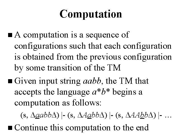
Computation n. A computation is a sequence of configurations such that each configuration is obtained from the previous configuration by some transition of the TM n Given input string aabb, the TM that accepts the language a*b* begins a computation as follows: (s, aabb ) |- (s, AAbb ) |- … n Continue this computation to the end

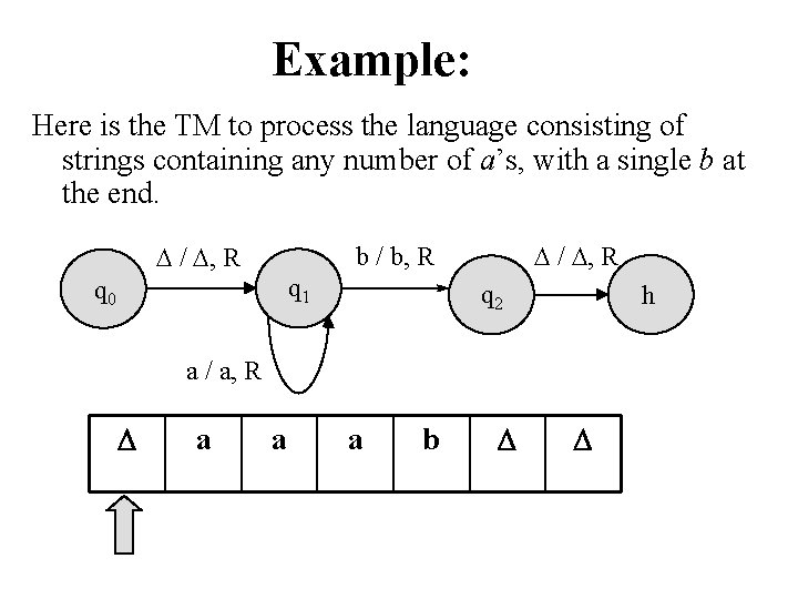
Example: Here is the TM to process the language consisting of strings containing any number of a’s, with a single b at the end. / , R b / b, R q 1 q 0 q 2 h a / a, R a a a b

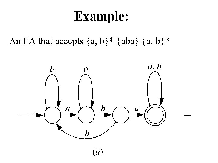
Example: An FA that accepts {a, b}* {aba} {a, b}*

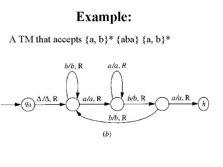
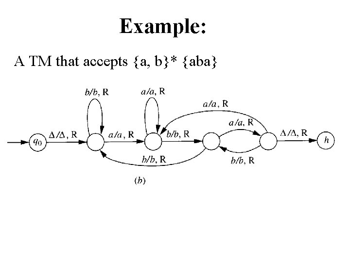
Example: A TM that accepts {a, b}* {aba} {a, b}*

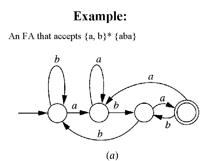
Example: An FA that accepts {a, b}* {aba}

Example: A TM that accepts {a, b}* {aba}

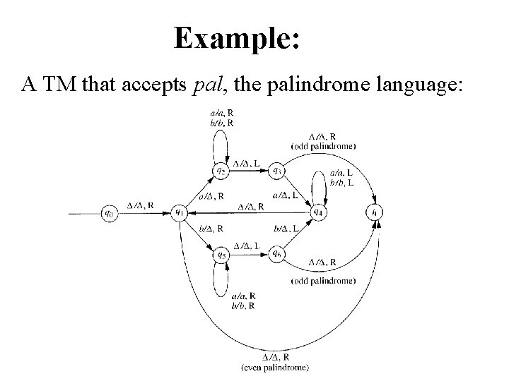
Example: A TM that accepts pal, the palindrome language:

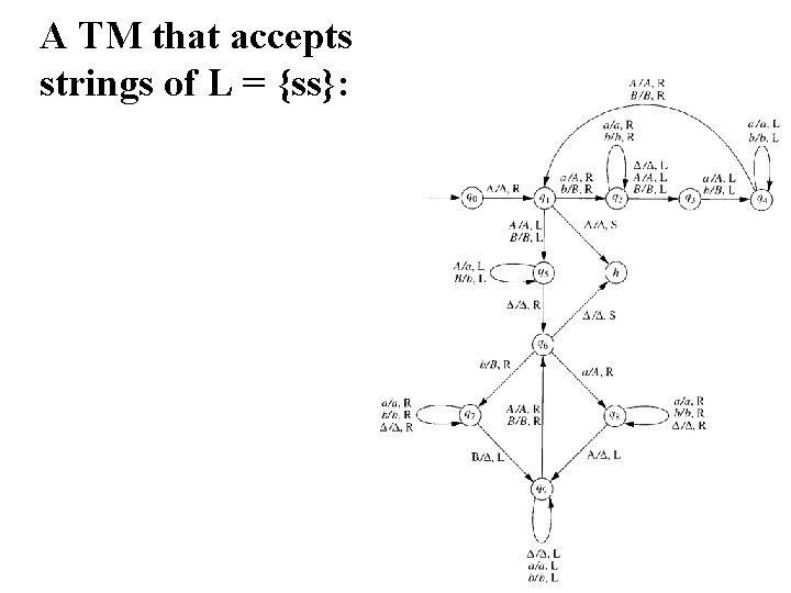
A TM that accepts strings of L = {ss}:

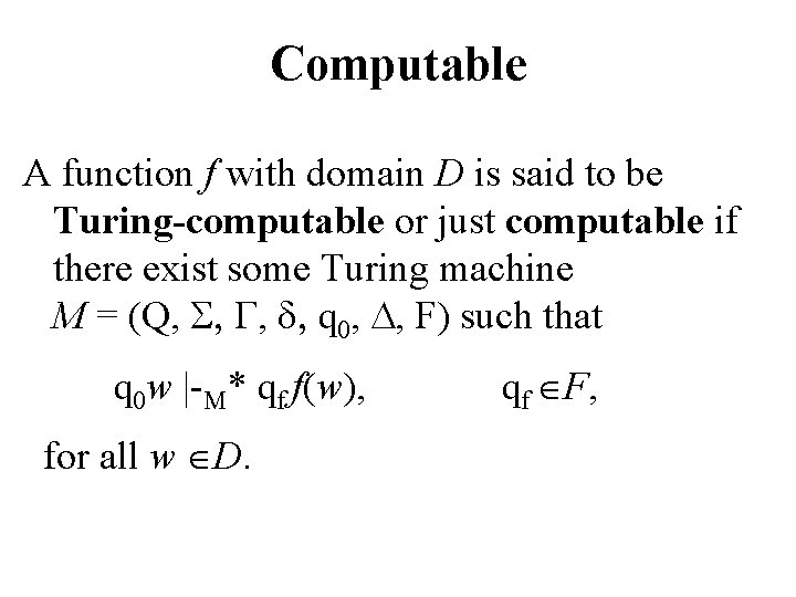
Computable A function f with domain D is said to be Turing-computable or just computable if there exist some Turing machine M = (Q, S, , , q 0, , F) such that q 0 w |-M* qf f(w), for all w D. qf F,

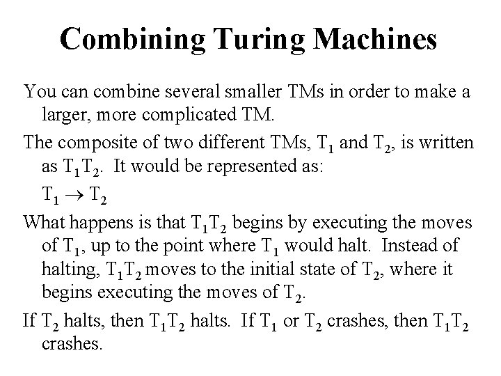
Combining Turing Machines You can combine several smaller TMs in order to make a larger, more complicated TM. The composite of two different TMs, T 1 and T 2, is written as T 1 T 2. It would be represented as: T 1 T 2 What happens is that T 1 T 2 begins by executing the moves of T 1, up to the point where T 1 would halt. Instead of halting, T 1 T 2 moves to the initial state of T 2, where it begins executing the moves of T 2. If T 2 halts, then T 1 T 2 halts. If T 1 or T 2 crashes, then T 1 T 2 crashes.

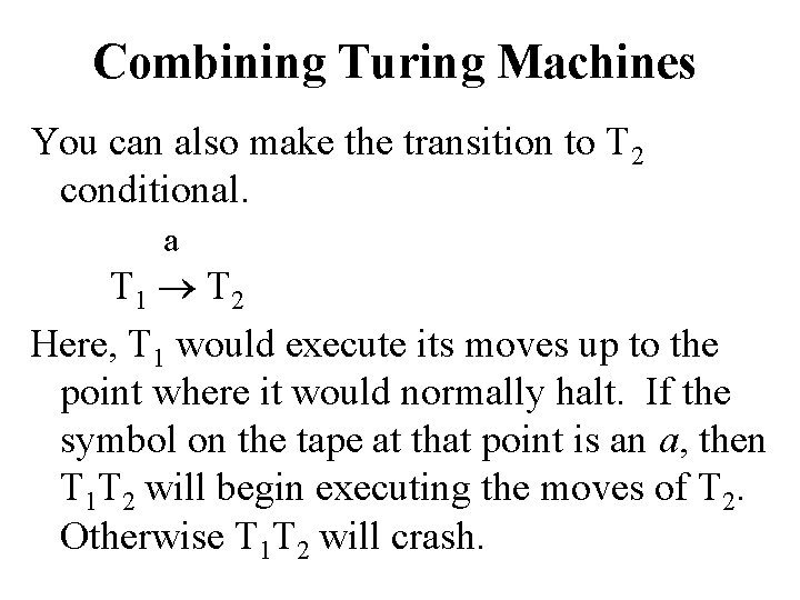
Combining Turing Machines You can also make the transition to T 2 conditional. a T 1 T 2 Here, T 1 would execute its moves up to the point where it would normally halt. If the symbol on the tape at that point is an a, then T 1 T 2 will begin executing the moves of T 2. Otherwise T 1 T 2 will crash.

Designing complex Turing machines n The book describes a “language” for combining simple TMs into complex ones, using the sequence, branching, and looping operators of imperative programming languages. n If you were going to be a Turing machine programmer, this would be useful. But …. n So, you will not be tested on this. But you need to understand how a Turing machine works and how to design simple ones.

Computing functions We use automata to recognize languages and compute functions (although we haven’t talked about computing functions until now). n In fact, computing functions allows language recognition, since every language can be represented by a characteristic function – if the input string is in the language, output 1 – otherwise output 0 n

String and numeric functions n n A TM can compute functions on strings. Given an input string, the output of the function is the string left on the tape after the TM halts. A TM can also compute numeric functions. Using a binary alphabet for strings, the input string can represent a binary number and the output string can represent a binary number. A TM can compute a function with multiple arguments. Each argument is separated by a blank on the tape. We can create TMs that compute arithmetic functions such as addition, subtraction, multiplication, etc.

Computing a Partial Function A Turing Machine can compute a function by leaving a string on the tape when it enters the halt state. A partial function f on S*may be undefined at certain points (the points not in the domain of f). A total function enters the halt state for all inputs in the domain. We say that a TM, T, computes f if T halts where f is defined and fails to halt elsewhere. So f is Turingcomputable, or just computable, if there exists some TM computing f.

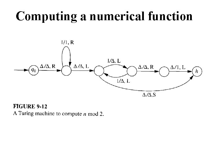
Computing a numerical function We can represent numbers on a TM by using the unary representation, which just uses n 1’s to represent the number n. Example: 11111 = 5 We can construct a TM to concatenate two strings together. If we represent two numbers in unary form, then a TM which concatenates these two strings is actually performing addition!

Computing a numerical function n The addition of two numbers is as simple as the concatenation of two strings. n Assume two integers are represented in unary form on the tape of a Turing machine. n Assume the two integers are separated by a 0 between them. n Design a Turing machine that will add these two numbers.

Computing a numerical function

Characteristic Function Computing the characteristic function L is very similar to accepting a language. The TM must always halt. The TM will leave a 1 on the tape if the string is accepted, and a 0 otherwise. HOWEVER: A TM can accept a language if it halts on all strings that are in the language, but doesn't halt on strings which are not.

Characteristic function: In a standard TM, strings which are not accepted can cause the TM to: • crash if it enters a state where there are no transitions for the current tape symbol, • crash if it tries to move left at the left end of the tape, or • get into an infinite loop, A TM computing the characteristic function must halt on all inputs

Conclusion Anything that is effectively calculable can be executed on a TM. A universal TM can compute anything that any other Turing machine can compute. The universal TM is itself a standard TM. A CPU with RAM is a finite version of a TM; it has the power of a TM up to the point that it runs out of memory. Languages or hardware that provides compares, loops, and increments are termed Turing complete and can also compute anything that is effectively calculable.