CSE 3813 Introduction to Formal Languages and Automata

CSE 3813 Introduction to Formal Languages and Automata Chapter 14 An Introduction to Computational Complexity These class notes are based on material from our textbook, An Introduction to Formal Languages and Automata, 4 th ed. , by Peter Linz, published by Jones and Bartlett Publishers, Inc. , Sudbury, MA, 2006. They are intended for classroom use only and are not a substitute for reading the textbook.

Can we solve it efficiently? We have seen that there is a distinction between problems that can be solved by a computer algorithm and those that cannot n Among the class of problems that can be solved by a computer algorithm, there is also a distinction between problems that can be solved efficiently and those that cannot n To understand this distinction, we need a mathematical definition of what it means for an algorithm to be efficient. n

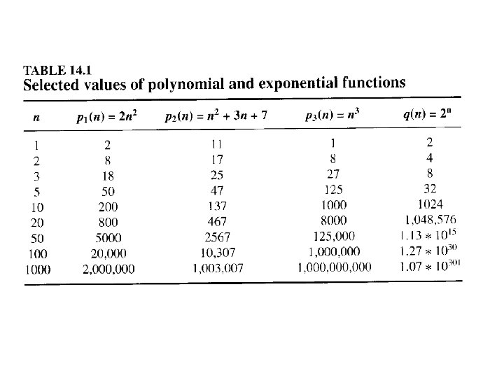
Growth Rates of Functions Different functions grow at different rates. For example:

Polynomial vs. exponential As you can see, there are some differences in how fast functions of different polynomials expand. The n 3 function gets bigger faster than either of the n 2 functions; its growth rate is bigger. However, these differences are insignificant compared to the differences between the any of the polynomial functions and the exponential function. For large values of n, 2 n is always greater than n 2. So usually we just lump all of the polynomial functions together, and distinguish them from the exponential functions.

Time and space complexity Theoretical computer scientists have considered both the time and space complexity of computational problems, in considering whether a problem can be solved efficiently. n For a Turing machine, time complexity is the number of computational steps required to solve a problem. Space complexity is the amount of tape required to solve the problem. n Both time and space complexity are important, but we will focus on the question of time complexity. n

Time and space complexity of a TM The time complexity of a TM is a measure of the maximum number of moves that the TM will require to process an input of length n. The space complexity of a TM is a measure of the maximum number of cells that the TM will require to process an input of length n. (Infinite loops excepted in either case. )

Basic complexity classes Time(f) is the set of languages that can be recognized by a TM T with a time complexity f. Space(f) is the set of languages that can be recognized by a TM T with a space complexity f. NTime(f) is the set of languages that can be accepted by an NTM T with nondeterministic time complexity f. NSpace(f) is the set of languages that can be accepted by a TM T with a nondeterministic space complexity f.

Basic complexity classes We can show that, for any function f: Time(f) NTime(f) and Space(f) NSpace(f). In addition, for any function f: Time(f) Space(f) and NTime(f) NSpace(f).

Theorem: We can show that, for any function f: NTime(f) Time(cf) This means that if we have an NTM that accepts L with nondterministic time complexity f, we can eliminate the nondeterminism at the cost of an exponential increase in the time complexity.

Worst-case time complexity The running time of a standard one-tape and onehead DTM is the number of steps it carries out on input w from the initial configuration to a halting configuration n Running time typically increases with the size of the input. We can characterize the relationship between running time and input size by a function n The worst-case running time (or time complexity) of a TM is a function f: N N where f(n) is the maximum number of steps it uses on any input of length n. n

Notation As you already know, we can use Big-O notation to specify the run-time for an algorithm. An algorithm for performing a linear search on a list requires a run time on the order of n, or O(n). A binary search on a sorted list of the same size requires a run time of O(log 2 n). There are other notations that also are commonly used, such as little-o, big theta, etc.

Asymptotic analysis n n n Because the exact running time of an algorithm is often a complex expression, we usually estimate it. Asymptotic analysis is a way of estimating the running time of an algorithm on large inputs by considering only the highest-order term of the expression and disregarding its coefficient. For example, the function f(n) = 6 n 3 + 2 n 2 + 20 n + 45 is aymptotically at most n 3. Using big-Oh notation, we say that f(n) = O(n 3). We will use this notation to describe the complexity of algorithms as a function of the size of their input.

Problem complexity n In addition to analyzing the time complexity of Turing machines (or algorithm), we want to analyze the time complexity of problems. n We establish in upper bound on the complexity of a problem by describing a Turing machine that solves it and analyzing its worst-case complexity. n But this is only an upper bound. Someone may come up with a faster algorithm.

The class P A Turing machine is said to be polynomially bounded if its running time is bounded by a polynomial function p(x p( ), where x is the size of the input. n A language is called polynomially decidable if there exists a polynomially bounded Turing machine that decides it. n The class P is the set of all languages that are polynomially decidable by a deterministic Turing machine. n

P is the same for every model of computation An important fact is that all deterministic models of computation are polynomially equivalent. That is, any one of them can simulate another with only a polynomial increase in running time. n The class P does not change if the Turing machine has multiple tapes, multiple heads, etc. , or if we use any other deterministic model of computation. n A different model of computation may increase efficiency, but only by a polynomial factor. n

Examples of problems in P n Recognizing any regular or context-free language. n Testing whethere is a path between points two points a and b in a graph. n Sorting and most other problems considered in a course on algorithms

Tractable Problems In general, problems that require polynomial time on a standard TM are said to be tractable. Problems for which no polynomial time algorithm is known for a TM are said to be intractable.

Deterministic vs. nondeterministic Remember that we can always convert a nondeterministic Turing machine into a deterministic Turing machine. Consequently, there is no difference in the absolute power of an NTM vs. a TM - either one can process any language that can be processed algorithmically.

Deterministic vs. nondeterministic However, when there are many alternative paths that the TM can follow in trying to process a string, only one of which leads to acceptance of the string, the NTM has the advantage to being able to automatically guess the correct sequence of steps to follow to accept a string, while the TM may have to try every possible sequence of steps until it finally finds the right one.

Deterministic vs. nondeterministic Thus, although an NTM isn’t more powerful than a TM, it may very well be faster on some problems than a TM.

P and NP If a deterministic Turing machine requires polynomial time to solve a problem (compute a function), then we say that this problem is in P, or that it is a P problem. P is therefore a set of problems (languages, functions) for which a p-time solution is known.

The class NP There are some problems for which no polynomialtime algorithm is known. These functions apparently require exponential time to execute on a Deterministic Turing Machine. However, they can be solved in polynomial time by an Nondeterministic Turing Machine. We call these problems NP problems (for Nondeterministic Polynomial). So NP also represents a set.

The class NP There are two ways to interpret what “can be solved in polynomial time on an NTM” means: 1. The NTM spawns off a clone of itself every time there is a new choice of paths to follow in processing a given string. 2. The TM has an oracle that guesses the right solution, and all the NTM has to do is to check it to see if it is correct.

The class NP n n n The class NP is the set of all languages that are polynomially decidable by a nondeterministic Turing machine. We can think of a nondeterministic algorithm as acting in two phases: – guess a solution (called a certificate) from a finite number of possibilities – test whether it indeed solves the problem The algorithm for the second phase is called a verification algorithm and must take polynomial time.

P and NP We know that P NP PSpace = NPSpace What is important here is that we know that P is a subset of NP, but we don’t know whether it is a proper subset or not. It may turn out to be the case that P = NP. We certainly don’t think so, but it hasn’t been proven either way.

NP-Reducibility One language, L 1, is polynomial-time reducible to another, L 2, if there is a TM with polynomial-time complexity that can convert the first language into the second. We write this as L 1 p L 2. Similarly, problems or functions may be Ptime reducible to other problems or functions.

NP-Hard and NP-Complete A language L is said to be NP-hard if L 1 p L for every L 1 NP. A language L is said to be NP-complete if L NP and L is NP-hard.

NP-complete problems n Informally, these are the hardest problems in the class NP n If any NP-complete problem can be solved by a polynomial time deterministic algorithm, then every problem in NP can be solved by a polynomial time deterministic algorithm n But no polynomial time deterministic algorithm is known to solve any of them

Examples of NP-complete problems n n n n Traveling salesman problem Hamiltonian cycle problem Clique problem Subset sum problem Boolean satisfiability problem The vertex cover problem The k-colorability problem Many thousands of other important computational problems in computer science, mathematics, economics, manufacturing, communications, etc.

Optimization problems and languages n n These examples are optimization problems. Aren’t P and NP classes of languages? We can convert an optimization problem into a language by considering a related decision problem, such as: Is there a solution of length less than k? The decision problem can be reduced to the optimization problem, in this sense: if we can solve the optimization problem, we can also solve the decision problem. The optimization problem is at least as hard as the decision problem.

Polynomial-time reduction Let L 1 and L 2 be two languages over alphabets 1 and 2, , respectively. L 1 is said to be polynomial-time reducible to L 2 if there is a total function f: 1* 2* for which 1) x L 1 if an only if f(x) L 2, and 2) f can be computed in polynomial time The function f is called a polynomial-time reduction.

Another view Polynomial-time reduction Set of instances of Problem Q’ One decision problem is polynomial-time reducible to another if a polynomial time algorithm can be developed that changes each instance of the first problem to an instance of the second such that a yes (or no) answer to the second problem entails a yes (or no) answer to the first.

A more interesting polynomial-time reduction n n The Hamiltonian cycle problem can be polynomial-time reduced to the traveling salesman problem. For any undirected graph G, we show to construct an undirected weighted graph G’ and a bound B such that G has a Hamiltonian cycle if and only if there is a tour in G’ with total weight bounded by B. Given G = (V, E), let B = 0 and define G’ = (V, E’) as the complete graph with the following weights assigned to edges: G has a Hamiltonian cycle if and only if G’ has a tour with total weight 0.

Examples of problem reductions SAT Is there a satisfying assignment for a proposition in conjunctive normal form? 3 -SAT Same as above except every clause in the proposition has exactly three literals. HAM-CYCLE TSP Given an undirected graph, determine whether it contains a Hamiltonian cycle (a path that starts at one node, visits every other node exactly once, and returns to start). Given a fully-connected weighted graph, find a least-weight tour of all nodes (cities).

SAT (Boolean satisfiability) In order to use polynomial-time reductions to show that problems are NP-complete, we must be able to directly show that at least one problem is NP-complete, without using a polynomial-time reduction n Cook proved that the Boolean satisfiability problem (denoted SAT) is NP-complete. He did not use a polynomial-time reduction to prove this. n This was the first problem proved to be NPcomplete. n

Definition of NP-Complete n. A problem is NP-Complete if 1. It is an element of the class NP 2. Another NP-complete problem is polynomial-time reducible to it n. A problem that satisfies property 2, but not necessarily property 1 is NP-hard.

Strategy for proving a problem is NPcomplete Show that it belongs to the class NP by describing a nondeterministic Turing machine that solves it in polynomial time. (This establishes an upper bound on the complexity of the problem. ) n Show that the problem is NP-hard by showing that another NP-hard problem is polynomialtime reducible to it. (This establishes a lower bound on the complexity of the problem. ) n

Complexity classes n n n n A complexity class is a class of problems grouped together according to their time and/or space complexity NC: can be solved very efficiently in parallel P: solvable by a DTM in poly-time (can be solved efficiently by a sequential computer) NP: solvable by a NTM in poly-time (a solution can be checked efficiently by a sequential computer) PSPACE: solvable by a DTM in poly-space NPSPACE: solvable by a NTM in poly-space EXPTIME: solvable by a DTM in exponential time

Relationships between complexity classes n n n NC P NP PSPACE = NPSPACE EXPTIME P EXPTIME Saying a problem is in NP (P, PSPACE, etc. ) gives an upper bound on its difficulty Saying a problem is NP-hard (P-hard, PSPACE-hard, etc. ) gives a lower bound on its difficulty. It means it is at least as hard to solve as any other problem in NP. Saying a problem is NP-complete (P-complete, PSPACE-complete, etc. ) means that we have matching upper and lower bounds on its complexity

P NP ? Theorem: If any NP-complete problem can be solved by a polynomial-time deterministic algorithm, then P = NP. If any problem in NP cannot be solved by a polynomial-time deterministic algorithm, then NP-complete problems are not in P. n This theorem makes NP-complete problems the focus of the P = NP question. n Most theoretical computer scientists believe that P NP. But no one has proved this yet. n

One of these two possibilities is correct NP NP-complete P NP NP NP-complete P

What does all this mean? For all practical purposes, if you know a problem is NP-complete, or if you can prove that it is reducible to one, then there is no point in looking for a P-time algorithm. You are going to have to do exponential-time work to solve this problem.

What should we do? Just because a problem is NP-complete, doesn’t mean we should give up on trying to solve it. n For some NP-complete problems, it is possible to develop algorithms that have average-case polynomial complexity (despite having worstcase exponential complexity) n For other NP-complete problems, approximate solutions can be found in polynomial time. Developing good approximation algorithms is an important area of research. n

Examples of NP-Complete Problems

Traveling salesman problem n Given a weighted, fully-connected undirected graph and a starting vertex v 0, find a minimal-cost path that begins and ends at v 0 and visits every vertex of the graph. n Think of the vertices as cities, arcs between vertices as roads, and the weights on each arc as the distance of the road.

Hamiltonian cycle problem A somewhat simplified version of the traveling salesman problem n Given an undirected graph (that has no weights), a Hamiltonian cycle is a path that begins and ends at vertex v 0 and visits every other vertex in the graph. n The Hamiltonian cycle problem is the problem of determining whether a graph contains a Hamiltonian cycle n

Clique problem n In an undirected graph, a clique is a subset of vertices that are all connected to each other. The size of a clique is the number of vertices in it. n The clique problem is the problem of finding the maximum-size clique in an undirected graph.

Subset sum problem n Given a set of integers and a number t (called the target), determine whether a subset of these integers adds up to t.

Boolean satisfiability problem n. A clause is composed of Boolean variables x 1, x 2, x 3, … and operators or and not. n Example: x 1 or x 2 or not x 3 n A Boolean formula in conjunctive normal form is a sequence of clauses in parentheses connected by the operator and. n Example: (not x 1 or x 2) and (x 3 or not x 2)

Boolean satisfiability n. A set of values for the variables x 1, x 2, x 3, … is called a satisfying assigment if it causes the formula to evaluate to true. n The satisfiability problem is to determine whether a Boolean formula is satisfiable.

Conclusion n You now know the difference between: – P and NP – NP-Hard and NP-Complete n You know the relationships between complexity classes n You know some examples of NP-Complete problems