Control PC Interface TE Port RRC PDCP RLC

 36.")

 PGW (PDN")
 Paging")
 PGW (PDN Gateway)")


 Video")
 HSS PCRF MME e. Node. B UE Other")
 AUTHENTICATION REQUEST 100 Trying")


 Tracking Area Update Request Old GUTI EPS Bearer")
 NAS(ESM) Message Type (8 bits) Protocol Discriminator + Message")


 (b) (c) (d) (e) 1 subframe")


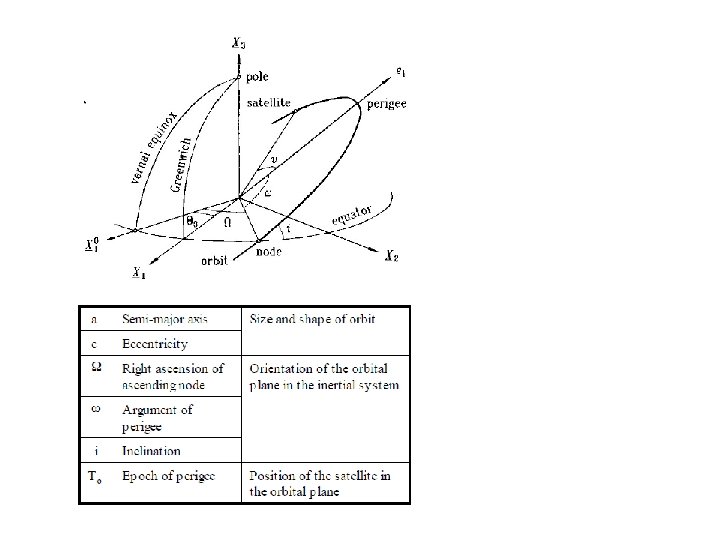
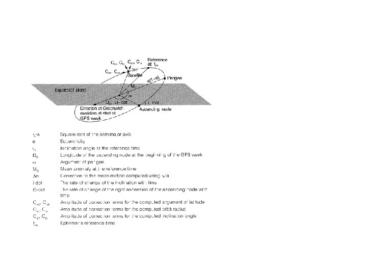
 Satellite clock, GPS")
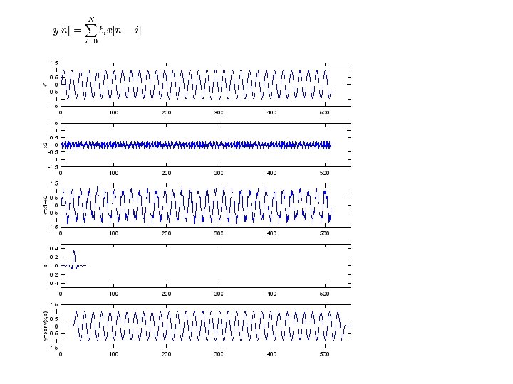
 y(n) x(n)y(n)")
 Correlation Inner Product Discrete Fourier Transform Convolution")
")

 with the size =")


 (x 1, y 1) 1. 0 0. 0 x 1")
 (x 1, y 1) -1. 0 0. 0 x 1")
 -1. 0 0. 0 x 1 x 2 0. 0")
 (x 2, y 2) cos(pi/4) -sin(pi/4) x 1 x 2")

 (a_f) (b_f) (c) Location, Size of the peak does not change, but graph")
")
 Abs(fft(s(t)) Arg(fft(s(t)) Abs(fft(s(t)) : Expanded Arg(fft(s(t)) : Expanded a b")


 (b) (c) Discontinuity of Phase Due to phase calculation software algorithm (d)")

 + cos()) Time")


 Modeling Algebra Laplace Transform F(s) (Laplace Form) Solving Solution Real")


 Any Solution Process Differential Equation e. g,")


 Voltage Drop (negative sign) Differentiate both sides Simplify the equation")


 =arg(a+b i) =angle of (a+b i) Real axis")

 Horizontal axis is automatically set, because it is not specified in plot() function")
 Total horizontal range is automatically set, because it is not specified in")
![plot(x, y); xlim([-8 8]); ylim([-1. 5]);](https://slidetodoc.com/presentation_image_h/8a5412ee965f79d25cdf46403e40d882/image-104.jpg "plot(x, y); xlim([-8 8]); ylim([-1. 5]);")
![plot(x, y); axis([-8 8 -1. 5]);](https://slidetodoc.com/presentation_image_h/8a5412ee965f79d25cdf46403e40d882/image-105.jpg "plot(x, y); axis([-8 8 -1. 5]);")
![plot(x, y); axis([-8 8 -1. 5]); title('y=sin(x)'); xlabel('x'); ylabel('sin(x)');](https://slidetodoc.com/presentation_image_h/8a5412ee965f79d25cdf46403e40d882/image-106.jpg "plot(x, y); axis([-8 8 -1. 5]); title('y=sin(x)'); xlabel('x'); ylabel('sin(x)');")
![color : ‘red’ format: ‘dashed line graph’ plot(x, y, ’r--’); axis([-8 8 -1. 5]);](https://slidetodoc.com/presentation_image_h/8a5412ee965f79d25cdf46403e40d882/image-107.jpg "color : ‘red’ format: ‘dashed line graph’ plot(x, y, ’r--’); axis([-8 8 -1. 5]);")
![plot(x, y 1, 'r-', x, y 2, 'b-'); axis([-8 8 -1. 5]);](https://slidetodoc.com/presentation_image_h/8a5412ee965f79d25cdf46403e40d882/image-108.jpg "plot(x, y 1, 'r-', x, y 2, 'b-'); axis([-8 8 -1. 5]);")
; plot() Subplot(M, N,")
![subplot(2, 2, 1); plot(x, y 1, 'r-'); axis([-8 8 -1. 5]); subplot(2, 2, 2);](https://slidetodoc.com/presentation_image_h/8a5412ee965f79d25cdf46403e40d882/image-110.jpg "subplot(2, 2, 1); plot(x, y 1, 'r-'); axis([-8 8 -1. 5]); subplot(2, 2, 2);")
 (the line")


- Slides: 121
Control PC Interface TE Port RRC PDCP RLC MAC PHY
Control PC Interface TE Port RRC 36. 331 PDCP 36. 323 Cpdcp. XXXXX() 36. 322 Crlc. XXXXX() RLC 36. 321 Cmac. XXXXX() MAC Cphy. XXXXX() 36. 104, 36. 211, 36. 212 36. 213, 36. 214, 36. 302 PHY Cte. XXXXX()
Protocol CT RF CT 36. 523 36. 521 -1, 36. 521 -3 23. 401, 24. 301, 29. 274, 32. 426, 33. 102, 33. 401, 33. 402 NAS 36. 331 RRC 36. 323 PDCP 36. 322 RLC 36. 321 MAC 36. 104, 36. 211, 36. 212 36. 213, 36. 214, 36. 302 PHY
SGSN PCRF HSS MME IP e. Node. B UE SGW (Serving Gateway) PGW (PDN Gateway)
MSC Voice Call Traffic Path Registration to CS Network Path BSC BTS (GSM) Paging Path SGSN SGs RNC UE Node. B (UMTS) MME IP e. Node. B (LTE) SGW (Serving Gateway) PGW (PDN Gateway)
SGSN PCRF HSS MME IP e. Node. B SGW (Serving Gateway) PGW (PDN Gateway) UE EPS Bearer External Bearer
UE Internet EPC E-UTRAN e. Node. B S-GW Peer Entity P-GW End-to-End Service EPS Bearer E-RAB External Bearer S 5/S 8 Bearer Radio Bearer S 1 Bearer Radio S 1 S 5/S 8 Gi
ON Duration DRX Cycle PDCCH Reception Here DRX Inactivity Time ON Duration DRX Cycle
PDCCH Reception Here DRX Inactivity Time ON Duration DRX Cycle DRX Command MAC CE Reception Here (Both DRX Inactivity timer and On. Duration Timer stops here) ON Duration Short DRX Cycle Timer Long DRX Cycle
http: //lteworld. org/blog/measurements-lte-e-utran High frequency Current Cell UE Center frequency Low frequency High frequency Center frequency Low frequency Target Cell
High frequency Current Cell UE Target Cell Center frequency Low frequency Target Cell High frequency Current Cell Center frequency Low frequency UE
High frequency Current Cell UE Target Cell Center frequency Low frequency High frequency Current Cell Center frequency Low frequency UE Target Cell
High frequency Current Cell UE Target Cell Center frequency Low frequency High frequency Current Cell UE Center frequency Target Cell Low frequency
IMS SIP H. 323 H. 263 RTP etc SMS Voice (Vo. IP) Video
SIP Application Servers SGSN IMS (CSCF) HSS PCRF MME e. Node. B UE Other IP Network SGW (Serving Gateway) PGW (PDN Gateway)
SIP Register Server Clients B A INVITE REGISTER (Contact Address) AUTHENTICATION REQUEST 100 Trying 180 Ringing 200 OK REGISTER (Credentials) Media Transfer OK BYE 200 OK
PC 1 – UE PC PC 2
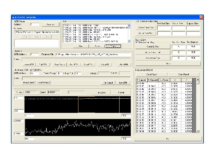
Server PC Ethernet Cable TE Port RF Port LTE Network Simulator UE PC Wireshark
Dummy Hub IP Network Data Server Router TE Port RF Port LTE Network Simulator Wireshark IP Monitoring PC for troubleshot UE PC Wireshark
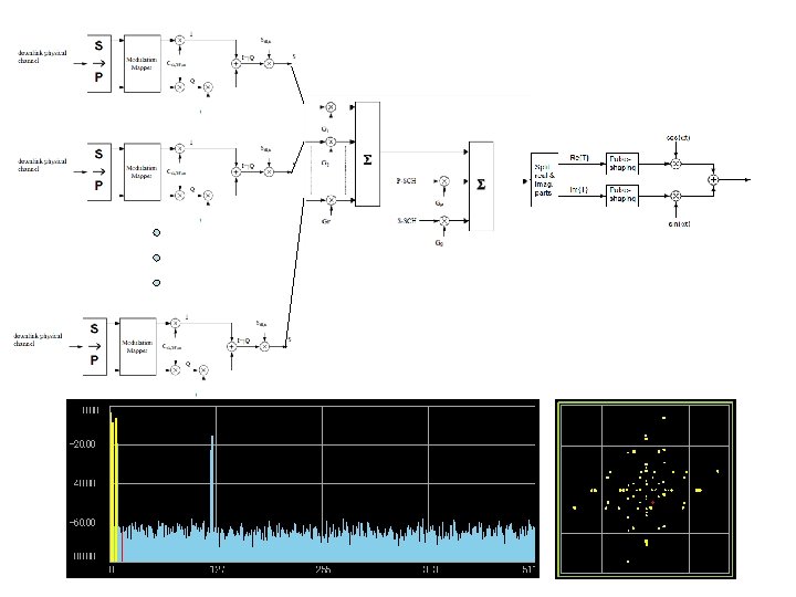
Bit Stream 36. 211 6. 3. 1 I/Q 36. 211 6. 3. 2 I/Q 36. 211 6. 3. 3 I/Q 36. 211 6. 3. 4 36. 211 6. 5
Cell Specific Reference Signal PDCCH PA PB PDSCH : in the same symbol as reference signal PDSCH : in the symbol with no reference signal
In some subframe, there can be no SRS depending on SRS Scheduling parameter settings 1 subframe
Attach Request EPS attach type value Old GUTI or IMSI PDN Connectivity Request PDN type Access point name UE network capability NAS : Security Mode Command Replayed UE security capabilities Attah Accept Activate Default EPS Bearer Setup Request GUTI PDN type EPS attach result value Access point name
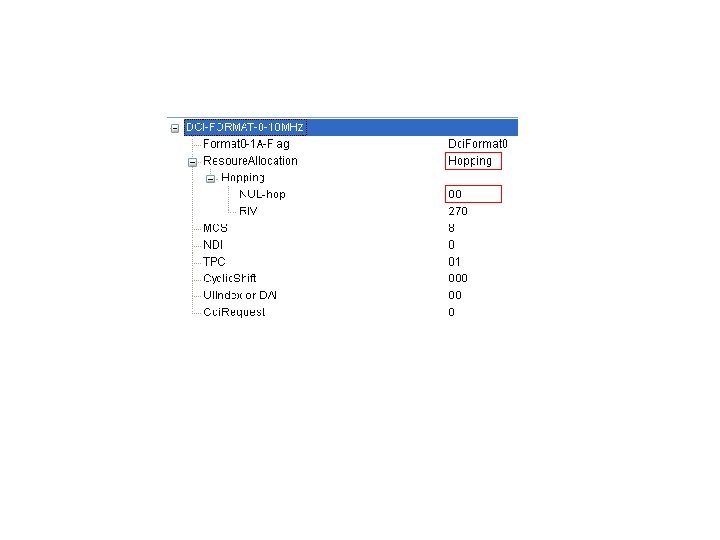
SIB 1 TAC (Tracking Area Code) Tracking Area Update Request Old GUTI EPS Bearer Context Status Old Location Area Identification Tracking Area Update Accept GUTI TAI List EPS Bearer Context Status Location Area Identification
RRC Dedicated. Info. NAS Message(EMM) NAS(ESM) Message Type (8 bits) Protocol Discriminator + Message Authentication Code + Sequence Number (44 bits) Security Header Type (4 bits) Length of Dedicated. Info. NAS C 1 (RRC Message Type Identifier : 4 bits)
1 frame 1 subframe 1 slot PUCCH Region Subband 3 Subband 2 Subband 1 Subband 0 PUCCH Region
PUCCH Region Subband 3 Subband 2 Subband 1 Subband 0 PUCCH Region
PUCCH Region Subband 3 Subband 2 Subband 1 Subband 0 PUCCH Region
PUCCH Region Subband 3 Subband 2 Subband 1 Subband 0 PUCCH Region
PUCCH Region Subband 3 Subband 2 Subband 1 Subband 0 PUCCH Region
PUCCH Region Subband 3 Subband 2 Subband 1 Subband 0 PUCCH Region
(a) (b) (c) (d) (e) 1 subframe
LTE CDMA WCDMA Voice Comm CSFB Packet Comm CSFB HO Packet Comm RD RD Idle HO CR CS RD CS Packet Comm RD CR Idle HO Packet Comm CR Idle CS CS Power On CS : Cell Selection CR : Cell Reselection RD : Cell Redirection HO : Handover CSFB : CS Fallback Idle
NW UE RRC Connection Request T 300 RRC Connection Setup NW UE RRC Connection Request T 300 RRC Connection Reject
UE Higher Layer UE Lower Layer Out of Sync Indication N 310 Times Out of Sync Indication In Sync Indication T 310 In Sync Indication N 311 Times In Sync Indication
UE Higher Layer UE Lower Layer Out of Sync Indication N 310 Times Out of Sync Indication T 310 Triggering Handover Procedure UE Higher Layer UE Lower Layer Out of Sync Indication N 310 Times Out of Sync Indication T 310 Initiating Connection Reestablishment
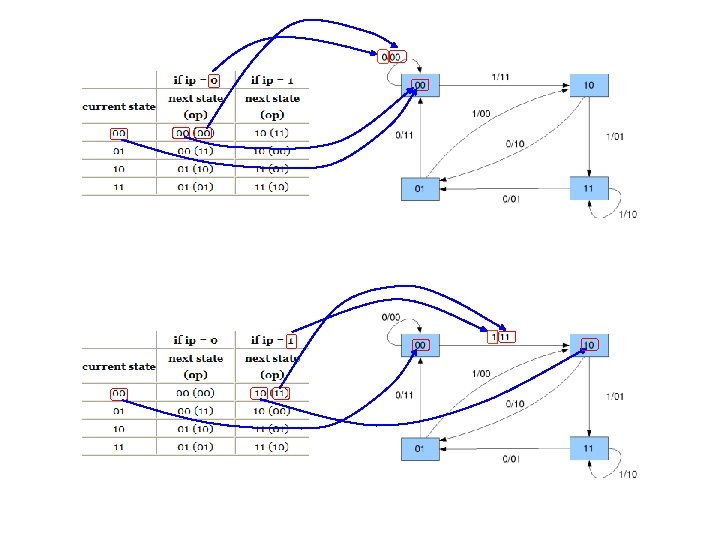
op 0 + 0 op + 0 0 ip 0 -1 Z 0 0 0 Z 0 -1 ip 0 + -1 Z 0 -1 + 0 1 + op op 1 + 0 0 ip 1 -1 Z 0 1 1 + Z 0 -1 ip 0 -1 Z 0 -1 + 1 op op
op 1 + 0 op + 1 0 ip 0 -1 Z 0 0 0 Z 1 -1 ip 1 + -1 Z 0 -1 + 1 op op op 1 + op 0 + 1 0 ip 1 -1 Z 0 1 1 + Z 1 -1 ip 1 -1 Z 0 -1 + 0 op op
op 0 + op 1 + 0 1 ip 0 -1 Z 1 0 0 + Z 0 -1 ip 0 -1 Z 0 Z 1 -1 + 0 1 + op op 0 + 0 1 ip 1 -1 Z 1 1 1 + Z 0 -1 ip 0 -1 Z 1 -1 + 1 op op
op 0 + 1 1 ip 0 -1 Z 1 0 0 + Z 1 -1 ip 1 -1 Z 0 Z 1 -1 + 1 1 + op op 1 + 1 1 ip 1 -1 Z 1 1 1 + Z 1 -1 ip 1 -1 Z 1 -1 + 0 op op
GPS Signal Frame Structure Telemetry and handover words (TLM and HOW) Satellite clock, GPS time relationship Telemetry and handover words (TLM and HOW) Ephemeris (precise satellite orbit) Telemetry and handover words (TLM and HOW) Almanac component (satellite network synopsys, error correction) Word Subframe 1 -2 3 -10 1 1 -2 3 -10 2 1 -2 3 Frame 300 bits 1500 bits 3 -10 4 5
x(n) y(n) x(n)y(n)
Sum of Times (Sum of Multiplication) Correlation Inner Product Discrete Fourier Transform Convolution
Sum of Times (Sum of Multiplication)
FIR IIR
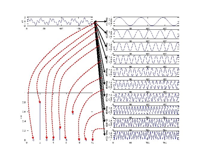
This means the result of convolution is an array (vector) with the size = n This means that each element (each value) of the convolution comes from “Sum of Multiplication” 1. 2. 3. 4. g[-m] This is same as g[-m + n] is same as g[-(m-n)] is same as g[-m] shifted by n g[-m] is the reflection of g[m] around y axis g[-(m-n)] =g[n-m] n g[m]
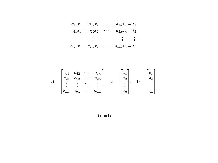
Control System Model Simultaneous Equations Matrix Statistics Operation / Manipulation Result Of Operation Graph Theory Statistics Graph Theory Computer Graphics Presentation Computer Graphics Linear Algegra Interpretation
(x 2, y 2) (x 1, y 1) 1. 0 0. 0 x 1 x 2 0. 0 1. 0 y 1 y 2
(x 2, y 2) (x 1, y 1) -1. 0 0. 0 x 1 x 2 0. 0 1. 0 y 1 y 2 1. 0 0. 0 x 1 x 2 0. 0 -1. 0 y 1 y 2 (x 1, y 1) (x 2, y 2)
(x 1, y 1) -1. 0 0. 0 x 1 x 2 0. 0 -1. 0 y 1 y 2 (x 2, y 2) (x 1, y 1) 1. 0 0. 3 x 1 x 2 0. 0 1. 0 y 1 y 2
(x 1, y 1) (x 2, y 2) cos(pi/4) -sin(pi/4) x 1 x 2 sin(pi/4) y 1 y 2 cos(pi/4) pi/4
0. 2 1 0. 8 0. 0 0. 4 0. 35 2 0. 15 0. 5 3 0. 6 To From 1 2 3 1 0. 2 0. 8 0. 0 2 0. 4 0. 15 0. 6 3 0. 5 0. 35 0. 0
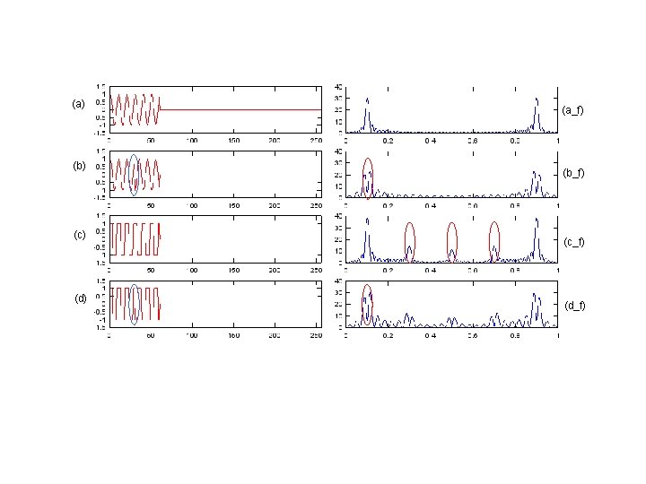
(a) (a_f) (b_f) (c) Location, Size of the peak does not change, but graph gets smoother (c_f) (d_f) Length of signal is same but lengh of Zero Pad gets longer Signal Zero Pad
Total number of data points is same but number of periods gets larger (a) (a_f) (b) (c) (b_f) Location of the peak does not change, but height of the peak gets higher and width of the peak (c_f) gets narrower (d) (d_f)
A B C s(t) Abs(fft(s(t)) Arg(fft(s(t)) Abs(fft(s(t)) : Expanded Arg(fft(s(t)) : Expanded a b c d e f g h i
a = 1. 0; b = 1. 0; p 1 = 0. 0; p 2 = 0. 0; A B C (a) (b) p (i) (iii) (c) (v) (d) (iv) Figure 1
a = 1. 0; b = 1. 0; p 1 = 0. 0; p 2 = 0. 2*pi; A B C (a) (b) p (i) (iii) (c) (v) (d) (iv) Figure 2
a = 1. 0; b = 0. 8; p 1 = 0. 0; p 2 = 0. 0; A B C (a) (b) p (i) (iii) (c) (v) (d) (iv) Figure 3 m 1 m 2
a = 1. 0; b = 0. 8; p 1 = 0. 0; p 2 = 0. 2*pi; A B C (a) (b) p (i) (iii) (c) (v) (d) (iv) Figure 4 m 1 m 2
(a) (b) (c) Discontinuity of Phase Due to phase calculation software algorithm (d)
A a = 1. 0; b = 1. 0; p 1 = 0. 0; p 2 = 0. 0; (a) (b) (c) (d) B a = 1. 0; b = 1. 0; p 1 = 0. 0; p 2 = 0. 2*pi; C a = 1. 0; b = 0. 7; p 1 = 0. 0; p 2 = 0. 0; D a = 1. 0; b = 0. 7; p 1 = 0. 0; p 2 = 0. 2*pi;
Time Domain Fourier Series Expansion A combination of infinite number (sin() + cos()) Time Domain Time domain Data Sequence Freq Domain Fourier Transform Frequency Domain Data
This is a differential equation because it has ‘derivative’ components in it derivative form differential form This is a differential equation because it has ‘differential’ components in it This is NOT a differential equation because it does not have ‘differential’ nor ‘derivative’ components in it This is NOT a differential equation because it is not a form of equation (no ‘equal’ sign) even though it has ‘derivative’ component in it
Algebraic Equation Solution Algebraic Equation Solver In this case, Variable y is a number In this case, Solution y is a value Differential Equation Solution Differential Equation Solver In this case, variable y is a function (e. g, y(x), y(t) etc)) In this case, Solution y is a function (e. g, y(x), y(t) etc))
As you see here, the dependent variable in differential equation is a ‘Function’, not a value. This is a key characteristics that defines ‘Differential Equation’ The highest order among all terms becomes the order of the differential equation. In this case, the highest Order is 3. So we call this equation as a ‘ 3 rd order differential equation’ Dependent Variable Independent Variable Order (=3) Order (=2) implies Independent Variable
Dependent Variable Independent Variable implies There are only one type of independent variable. This kind of differential equation is called Ordinary Differential Equation (ODE) Independent Variable Dependent Variable Independent Variable implies There are more than one types of independent variables. (In this example, we have two different type of independent variable). This kind of differential equation is called Partial Differential Equation (PDE) Independent Variable
Calculus Differential Equation (Continous) Modeling Algebra Laplace Transform F(s) (Laplace Form) Solving Solution Real World Problem Inverse Transform Solution Modeling Solving Difference Equation (Discrete) Solution F(z) (z Form) z Transform
Laplace Transform Symbols for original function Symbols for Laplace Transformed Function Definition of Laplace Transformed Function
: Unit Step 1
Differential Equation e. g, f(y’’, y’, t) Any Solution Process Differential Equation e. g, f(y’’, y’, t) Laplace Transform y(t) = ? ? ? Y(s) = ? ? ? Inverse Laplace Transform y(t) = ? ? ?
Derive a differential equation that tells you the velocity of a falling body at any given time. (Assume the condition where you should not ignore the air resistance) Governing Law : Total Force applied to a body = Motion of the body Q. Can I convert this into a term related to velocity ? Q. What kind of Force is there ? i) A. Yes. Acceleration (a) is the derivative of velocity (v) Force to helps movement = Pulling force by gravity = ii) Force to hinder movement = air resistance = Why negative sign here ? : It is because this fource act in opposite direction to the other Force (Gravity). : We assumed that Pulling Force by Gravity is ‘Positive Force’
A B C Force trying to get to the spring’s resting position = -k s p 4 p 1 s -x x=0 p 2 +x p 3 Force being pulled down by gravity =mg If you hand a mass to the spring, it would try to fall down and length of the spring would increase, but soon the mass would not fall down anymore because of the restoration force of the spring. This is the point where the springs restoration force and pulling force by gravity become same. We call this point as “Equilibrium Point”. At this point, the mass does not move in any direction. So it is the same situation where there is no force being applied to the body (in reality, the two force with the same amount is continuously being applied in opposite direction) It is very important to know where is the reference point, the point where we define x = 0. It is totally up to you how to define the reference point. You can set any point as a reference point but the final mathematical equation may differ depending on where you take as a reference point. So usually, we set the point where we can get a simplest mathematical model. In vertical spring model, we set the Equilibrium Point as the reference point because we can remove the term –k s and mg since they cancel each other at this point
C Governing Law : Total Force applied to a body = Motion of the body Q. What kind of Force is there ? i) -x A. x=0 +x Force to makes movement = Restoration force of the spring trying to get back to the equilibrium position = ii) Force created by Gravity = Force pulling the object down to the ground = iii) We can set this part to be ‘ 0’ by setting ‘the equilibrium point’ as the reference point of the model. (Refer to previous figure and comments on it) Q. Can I convert this into a term related to position of the mass (x = distance from the reference point) ? Force to oppose the pulling force by gravity = Restoration force of the spring just to oppose the pulling force by gravity = iv) Force to prevent movement = damping force = Yes. Acceleration (a) is the 2 nd derivative of distance (x)
Governing Law : Population Growth Rate per Individual = Rate of Factors increasing the Population – Rate of Factoring decreasing the Population Q. What kind of Factors are there ? i) Increasing Factors a) Birth Rate ? = b) Rate of immigration = ii) Decreasing Factors a) Death Rate = b) Rate of emigration =
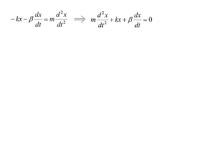
Governing Law : Kirchhoff's voltage law The directed sum of the electrical potential differences (voltage) around any closed circuit is zero The sum of the emfs in any closed loop is equivalent to the sum of the potential drops in that loop Voltage Drop EMFS : Voltage Generator Voltage Drop
Voltage Generator(positive sign) Voltage Drop (negative sign) Differentiate both sides Simplify the equation
Mathematical Operation Modeling Interpretation Other Models Differential Equation Real World Problem Matrix Statistics Probability (Stocastics) Other Models Mathematical Solution Real World Solution
amp 1 CH 1 x I amp 2 CH 2 x + amp 1 CH 3 x Q CH 4 amp 2 x x j I+j. Q
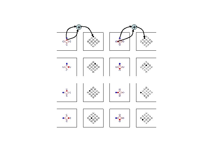
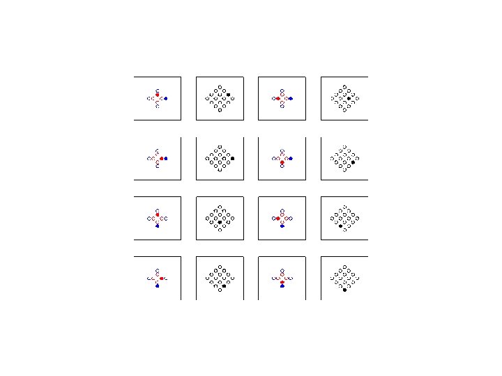
x 1 amplitude = 1 x 2 amplitued = 0. 5 x 1 amplitude = 1 x 2 amplitued = 0. 25 How do we get this kind of constellation ?
e 2 e 1 x 1 e 3 e 4 EVM_x 1 = min{e 1, e 2, e 3, e 4};
assuming Is this constellation correct ?
Chip Rate Signal
Real part Imaginary axis =abs(a+b i) =arg(a+b i) =angle of (a+b i) Real axis
c 3 = c 1 + c 2 c 1 c 3 c 1
plot(y) Horizontal axis is automatically set, because it is not specified in plot() function
plot(x, y) Total horizontal range is automatically set, because it is not specified in plot() function
plot(x, y); xlim([-8 8]); ylim([-1. 5]);
plot(x, y); axis([-8 8 -1. 5]);
plot(x, y); axis([-8 8 -1. 5]); title('y=sin(x)'); xlabel('x'); ylabel('sin(x)');
color : ‘red’ format: ‘dashed line graph’ plot(x, y, ’r--’); axis([-8 8 -1. 5]); title('y=sin(x)'); xlabel('x'); ylabel('sin(x)');
plot(x, y 1, 'r-', x, y 2, 'b-'); axis([-8 8 -1. 5]);
col 1 row 2 1 N+1 row M Subplot(M, N, 1); plot() Subplot(M, N, 2); plot() Subplot(M, N, 3); plot() Subplot(M, N, M x N); plot() col 2 col 3 col N 2 3 N N+2 N+3 N+N Nx. N
subplot(2, 2, 1); plot(x, y 1, 'r-'); axis([-8 8 -1. 5]); subplot(2, 2, 2); plot(x, y 2, 'g-'); axis([-8 8 -1. 5]); subplot(2, 2, 3); plot(x, y 3, 'b-'); axis([-8 8 -1. 5]); subplot(2, 2, 4); plot(x, y 4, 'm-'); axis([-8 8 -1. 5]);
re al Plot curve along imaginary axis (absolute value of the expression) (the line where real value = 0) = This represents ‘Frequency Response’ imaginary pole Plot curve along imaginary axis (arg of the expression) (the line where real value = 0)