EEE 302 Electrical Networks II Dr Keith E

EEE 302 Electrical Networks II Dr. Keith E. Holbert Summer 2001 Lecture 22 1

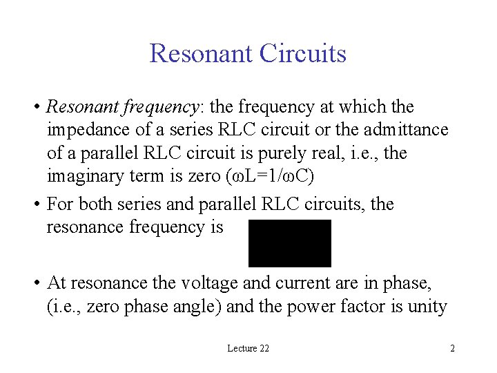
Resonant Circuits • Resonant frequency: the frequency at which the impedance of a series RLC circuit or the admittance of a parallel RLC circuit is purely real, i. e. , the imaginary term is zero (ωL=1/ωC) • For both series and parallel RLC circuits, the resonance frequency is • At resonance the voltage and current are in phase, (i. e. , zero phase angle) and the power factor is unity Lecture 22 2

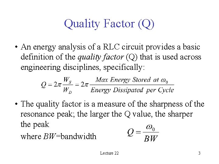
Quality Factor (Q) • An energy analysis of a RLC circuit provides a basic definition of the quality factor (Q) that is used across engineering disciplines, specifically: • The quality factor is a measure of the sharpness of the resonance peak; the larger the Q value, the sharper the peak where BW=bandwidth Lecture 22 3

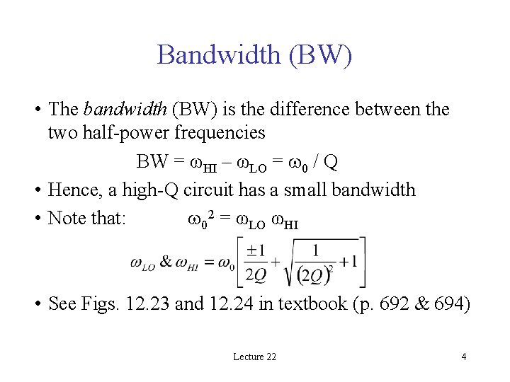
Bandwidth (BW) • The bandwidth (BW) is the difference between the two half-power frequencies BW = ωHI – ωLO = 0 / Q • Hence, a high-Q circuit has a small bandwidth • Note that: 02 = ωLO ωHI • See Figs. 12. 23 and 12. 24 in textbook (p. 692 & 694) Lecture 22 4

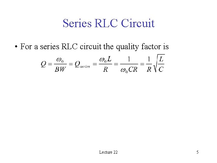
Series RLC Circuit • For a series RLC circuit the quality factor is Lecture 22 5

Class Examples • • • Extension Exercise E 12. 8 Extension Exercise E 12. 9 Extension Exercise E 12. 10 Extension Exercise E 12. 11 Extension Exercise E 12. 12 Lecture 22 6

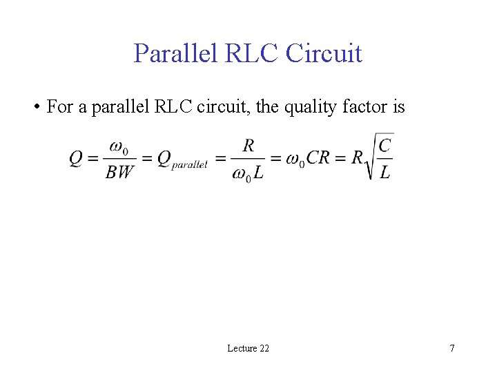
Parallel RLC Circuit • For a parallel RLC circuit, the quality factor is Lecture 22 7

Class Example • Extension Exercise E 12. 13 Lecture 22 8

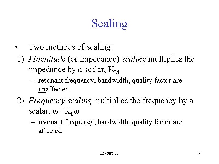
Scaling • Two methods of scaling: 1) Magnitude (or impedance) scaling multiplies the impedance by a scalar, KM – resonant frequency, bandwidth, quality factor are unaffected 2) Frequency scaling multiplies the frequency by a scalar, ω'=KFω – resonant frequency, bandwidth, quality factor are affected Lecture 22 9

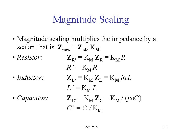
Magnitude Scaling • Magnitude scaling multiplies the impedance by a scalar, that is, Znew = Zold KM • Resistor: ZR’ = KM ZR = KM R R’ = KM R • Inductor: ZL’ = KM ZL = KM j L L’ = KM L • Capacitor: ZC’ = KM ZC = KM / (j C) C’ = C / KM Lecture 22 10

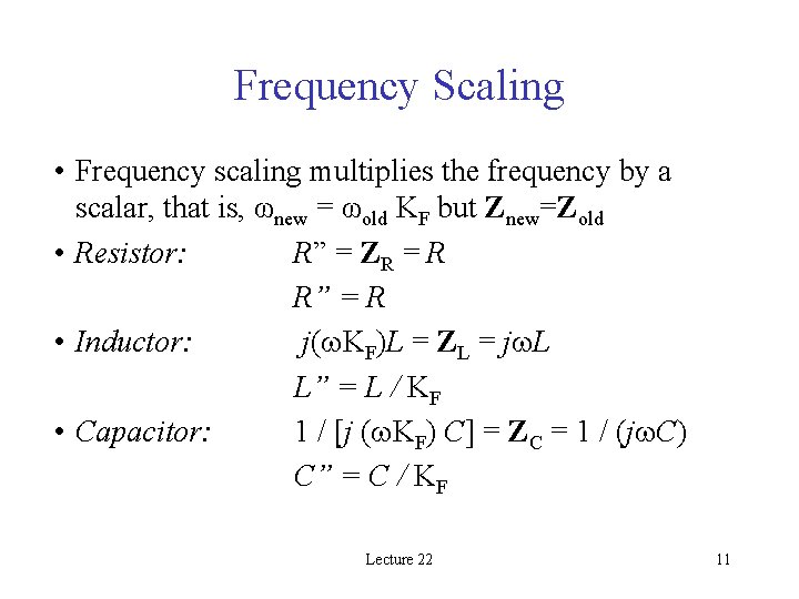
Frequency Scaling • Frequency scaling multiplies the frequency by a scalar, that is, ωnew = ωold KF but Znew=Zold • Resistor: R” = ZR = R R” = R • Inductor: j( KF)L = ZL = j L L” = L / KF • Capacitor: 1 / [j ( KF) C] = ZC = 1 / (j C) C” = C / KF Lecture 22 11

Class Example • Extension Exercise E 12. 15 Lecture 22 12