What is Gravity Method The gravity method involves

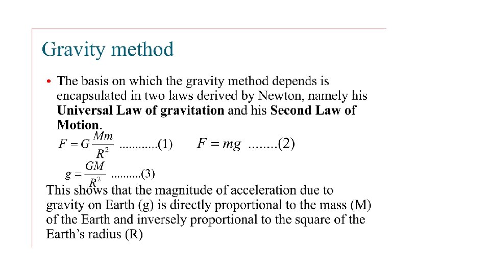
What is Gravity Method? The gravity method involves measuring the earth’s gravitational field at specific locations on the earth’s subsurface to determine the location of subsurface density variations. The gravity method involves measuring the gravitational attraction exerted by the earth at a measurement station on the surface. Geologists can make inferences about the distribution of strata.

The primary goal of studying detailed gravity data is to provide a better understanding of the subsurface.

Why Gravity Method used widely? Non-destructive geophysical technique Measures differences in the Earth’s gravitational field at specific locations Provides a better understanding of the subsurface geology Relatively cheap Non-invasive remote sensing method No energy need be put into the ground in order to acquire data Well suited to a populated setting

Applications of Gravity method in: • Engineering, Environmental and Geothermal studies including: • Locating voids, • Faults, • Buried stream valleys, • Water table levels and Geothermal heat sources • The thickness of the soil layer

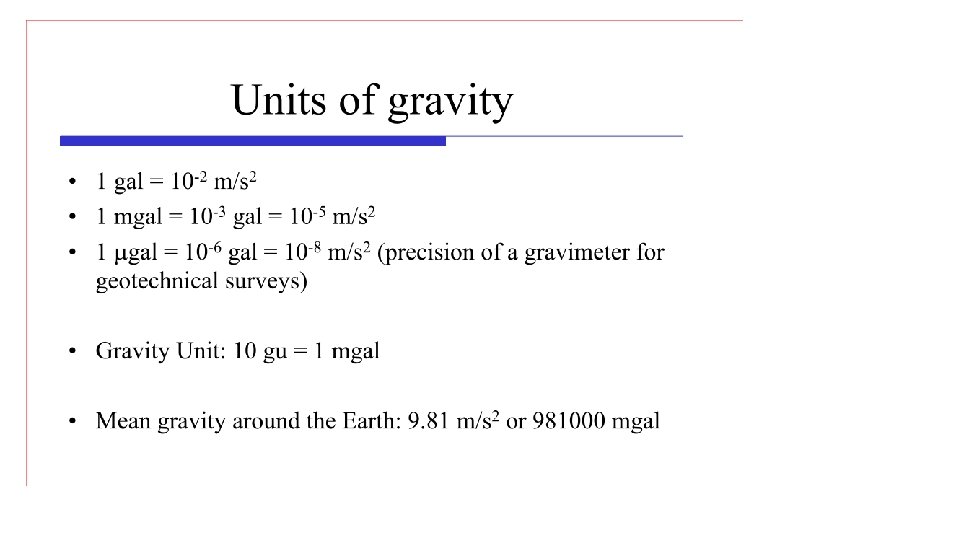
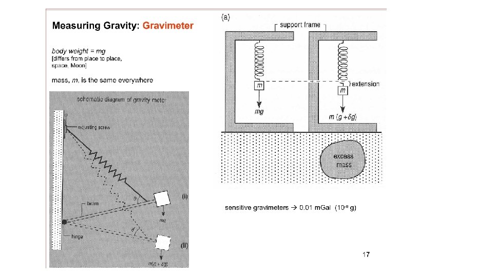
Units of gravity • • • The mean value of gravity at the Earth’s surface is about 9. 8 ms-2. Variations in gravity caused by density variations in the subsurface are of the order of 100 micro-ms-2. • This unit of the micrometer per second is referred to as the gravity unit (gu). In gravity surveys on land an accuracy of ± 0. 1 gu is readily attainable, corresponding to about one hundred millionth of the normal gravitational field. • At sea the accuracy obtainable is considerably less, about ± 10 gu. The c. g. s. unit of gravity is the milligal (1 mgal = 10 -3 cms-2), equivalent to 10 gu.

Gravity techniques measure minute variations in the earth's gravity field. Based on these variations, subsurface density and thereby composition can be inferred. These variations can be determined by measuring the earth's gravity field at numerous stations along a traverse, and correcting the gravity data for elevation, tidal effects, topography, latitude, and instrument drift.

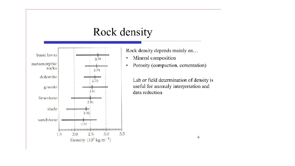
• The gravity field on the surface of the Earth is not uniformly the same everywhere. It varies with the distribution of the mass materials below. A Gravity survey is a direct means of calculating the density property of subsurface materials. • The higher the gravity values, the denser the rock beneath.

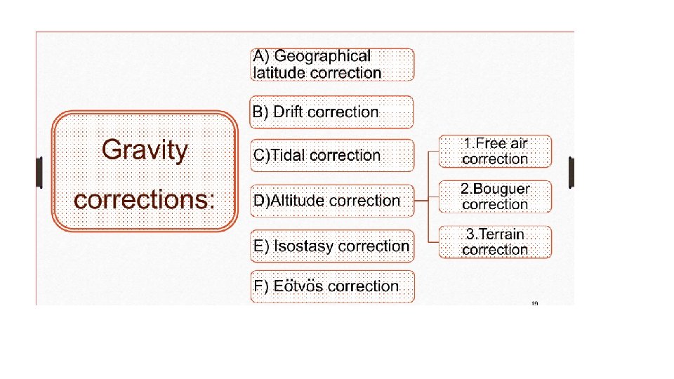
• Gravity Data Reductions • • Gravity values vary from place to place. Some of those variations have obvious causes such as earth flattening and rotation, variation in the distance from the earth’s centre, and the fact that there would appear to be more mass beneath a high gravity site than a lower one, causing the gravity values measured at these sites to differ. • By correcting for the above factors, (a process referred to as “reduction”) the remaining changes of gravity values will only depend on the density contrast relating to geological features or structures

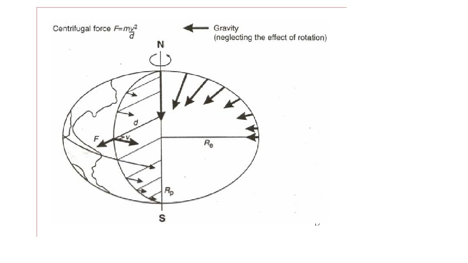
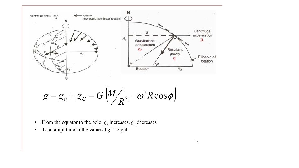
• Latitude correction • Variation of gravity with latitude is due to the none-spherical shape of the earth and the angular velocity variations from zero at the pole to its maximum at the equator (Kearey and Brooks 1991). Rotation generated centripetal acceleration causes the gravity to increase from equator to the pole. And effect that is partly counteracted by the larger radius at the equator than the pole. Never the less these remains a net increase of approximately 5186 m. Gal from equator to pole. Also the radius at the equator is longer than at the pole which is partly counteracted by the increased mass at the equator, but still caused the gravity to increase from the equator to pole the net result of the above two factors is approximately 5186 m. Gal increase of gravity at the pole with respect to the equator.

The latitude correction is determined by the Clairaut’s formula: This formula relates gravity to latitude on the reference spheroid, where Glat is theoretical gravity value at the latitude of the gravity reading. Gequator is the gravity value at the equator. K 1 and K 2 are constants dependent on the shape and speed of rotation of the earth. The resulting Glat should be subtracted from the observed value to correct for the latitude variation

• The Gravity formula was modified at least three times in this century in 1930, 1967 and 1984. In 1930 the first international accepted reference ellipsoid was established and its parameters were used for the 1930 International Gravity Formula: Glat=978049. 0(1+0. 0052884 sin 2(lat)-0. 0000059 sin 2 (2 xlat))

• However, by calculating more precise geodetic parameters from satellite observations the 1930 gravity formula was modified to the 1967 Geodetic Reference System Formula (GRS 67) Glat=978031. 846(1+0. 0053024 sin 2(lat)-0. 0000059 sin 2 (2 xlat))

• In 1979 the International Association of Geodesy (IAG) adopted the Geodetic Reference System 1980 (GRS 80) which led the World Geodetic System 1984 (WGS 84) and a theoretical gravity formula approximated by: • Glat=978032. 67714(1+0. 00193185138639 sin 2(lat)/(1 -0. 00669437999013 sin 2(lat))1/2

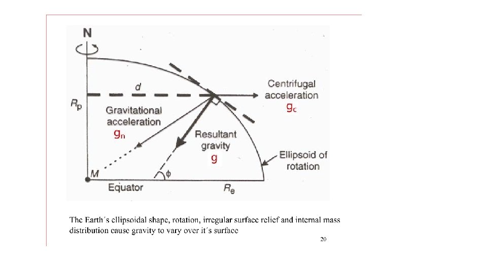
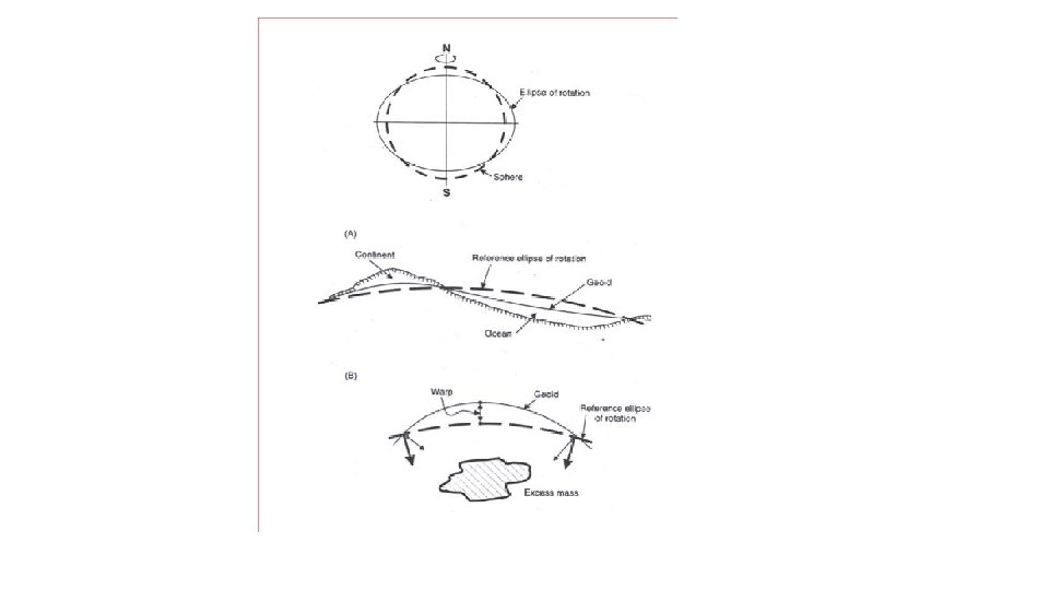
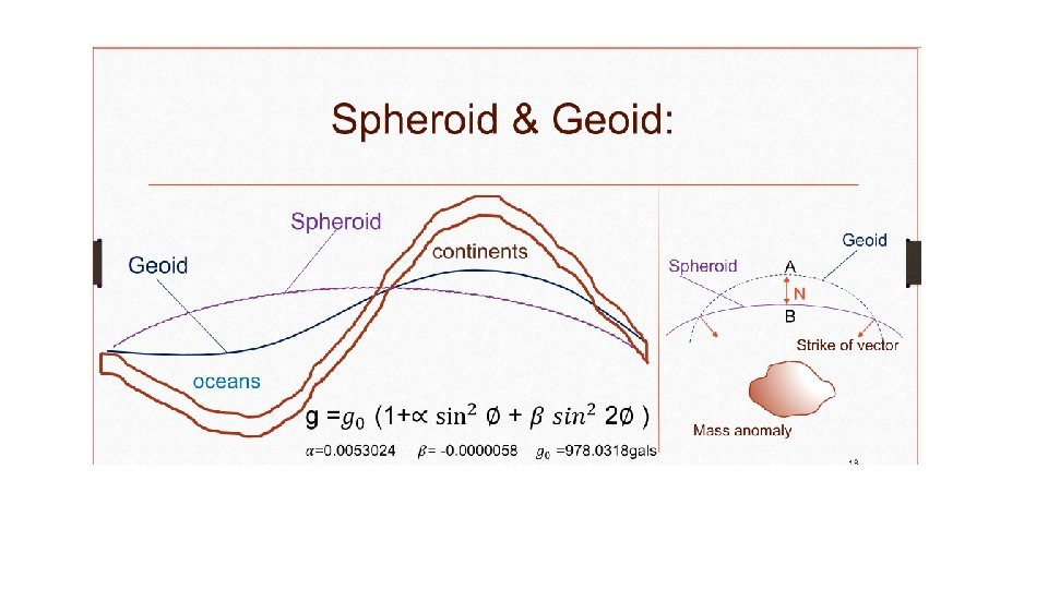
In summary Results of measurements of gravity (g) presented as deviations from mean value of gravity, the normal gravity or theoretical gravity Glat is called Normal gravity gn or theoretical gravity Average gravitational acceleration on the surface of the earth, gn depends on latitude gn greatest at the poles gn least at the equator

Latitude Correction • Correction from gobs that accounts for Earth's elliptical shape and rotation. The gravity value that would be observed if Earth were a perfect (no geologic or topographic complexities), rotating ellipsoid is referred to as the normal gravity. Gravity INCREASES with increasing latitude. Correction is ADDED as we move toward the equator. Correction is applied ONLY in the N-S direction

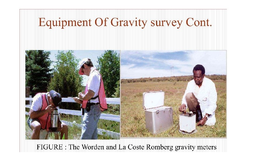
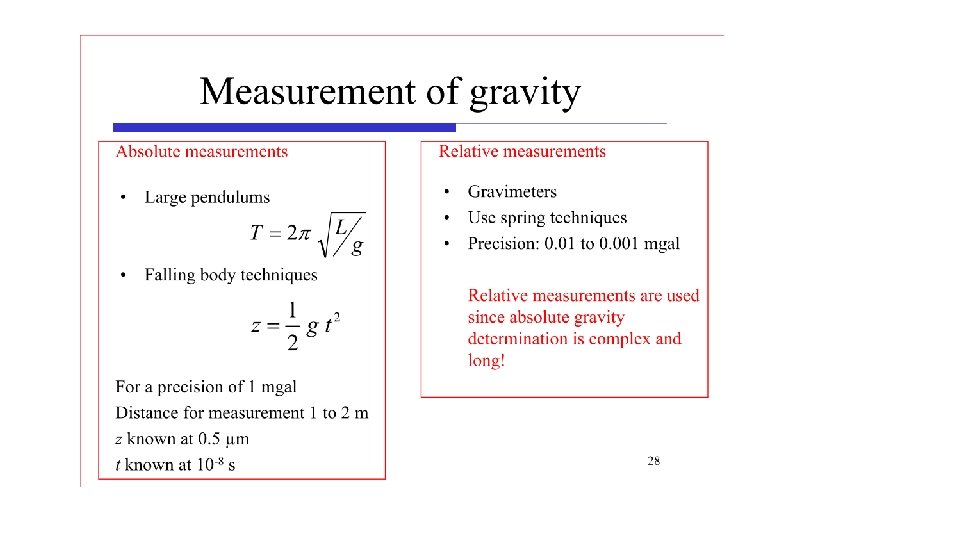
Equipment Of Gravity survey A gravity meter or gravimeter measures the variations in the earth's gravitational field. The most commonly used meters do not measure an absolute gravitational acceleration but differences in relative acceleration. The common gravimeters on the market are the Worden gravimeter, the Scintrex and the La Coste Romberg gravimeter. The Scintrex Autograv is semi-automated, but although a bit more expensive. The Lacoste and Romberg model gravity meter is one of the preferred instruments for conducting gravity surveys in industry.

Views of the Lacoste -Romberg Gravity Meter

CG 5 Scintrex

Drift correction • Correction for instrumental drift is based on repeated readings at a base station at recorded times throughout the day. The meter reading is plotted against time and drift is assumed to be linear between consecutive base readings.

From the figure drift is assumed to be linear between consecutive base readings. The drift correction at time t is d, which is subtracted from the observed value.

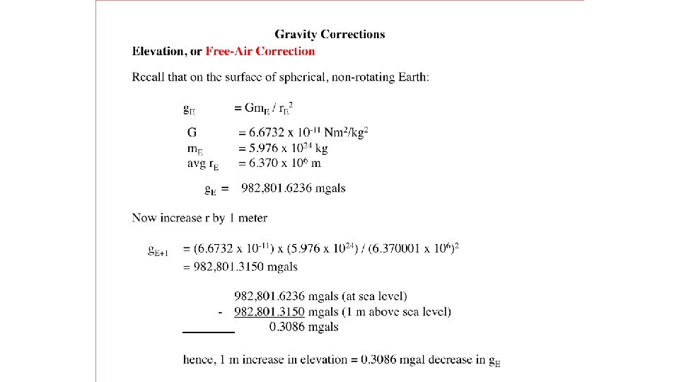
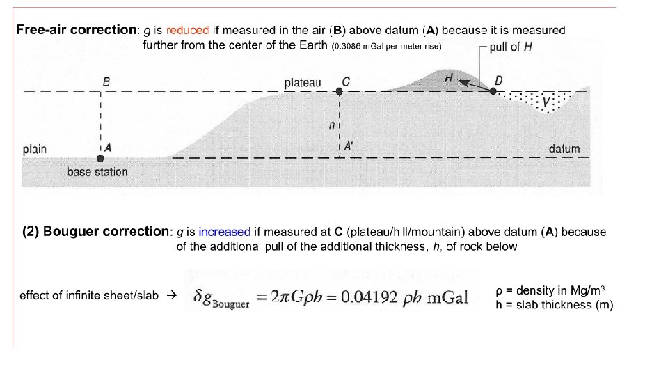
Free-Air Correction Often we make observations at different elevations, and we know that gravity will decrease as we get farther from the center of mass of the Earth. Therefore, we choose a reference elevation (typically sea level) and adjust our readings to be what they would be at that elevation. To compute this correction, recall that g = GM/r 2 And so dg/dr = -2 GM/r 3 = -2 g/r = -0. 3085 mgals/m = -0. 09406 mgals/ft.

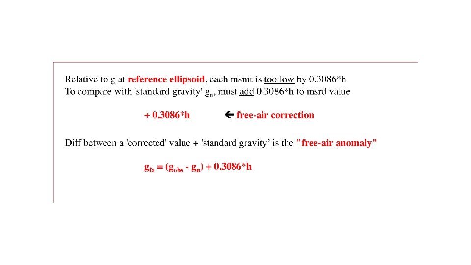
• The free-air correction (FAC) corrects for the decrease in gravity with height in free air resulting from increased distance from the centre of the Earth. • The FAC is positive for an observation point above datum to correct for the decrease in gravity with elevation. • The free-air correction accounts solely for variation in the distance of the observation point from the centre of the Earth; • no account is taken of the gravitational effect of the rock present between the observation point and datum.

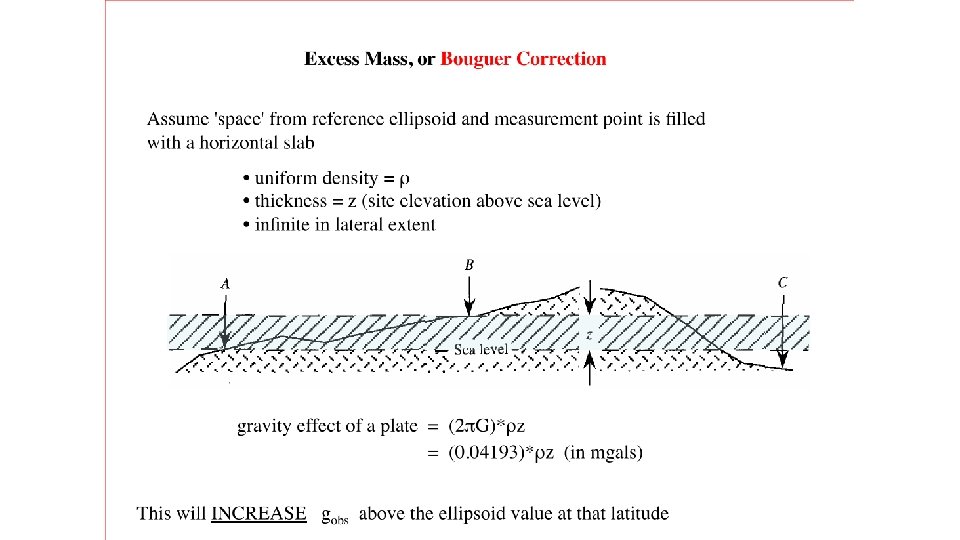
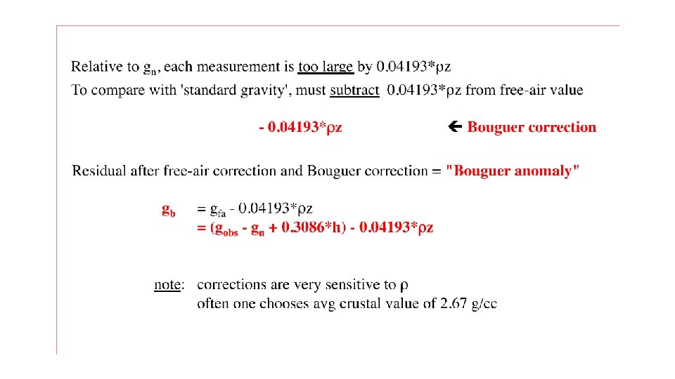
Bouguer correction • On land the Bouguer correction must be subtracted, as the gravitational attraction of the rock between observation point and datum must be removed from the observed gravity value. • The Bouguer correction of sea surface observations is positive to account for the lack of rock between surface and sea bed. The correction is equivalent to the replacement of the water layer by material of a specified rock density

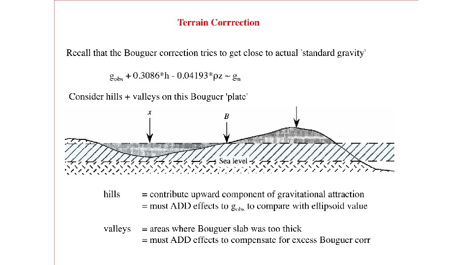
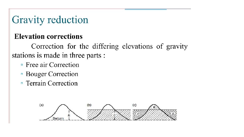
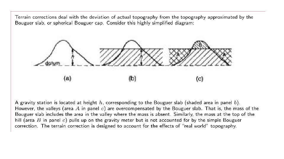
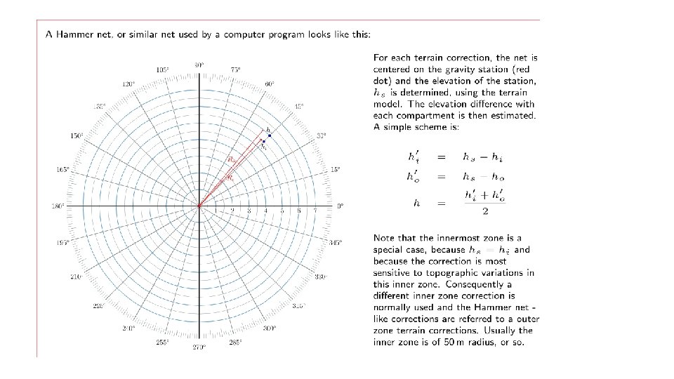
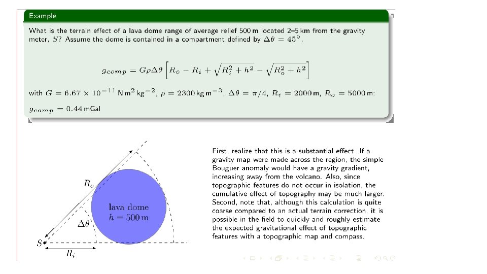
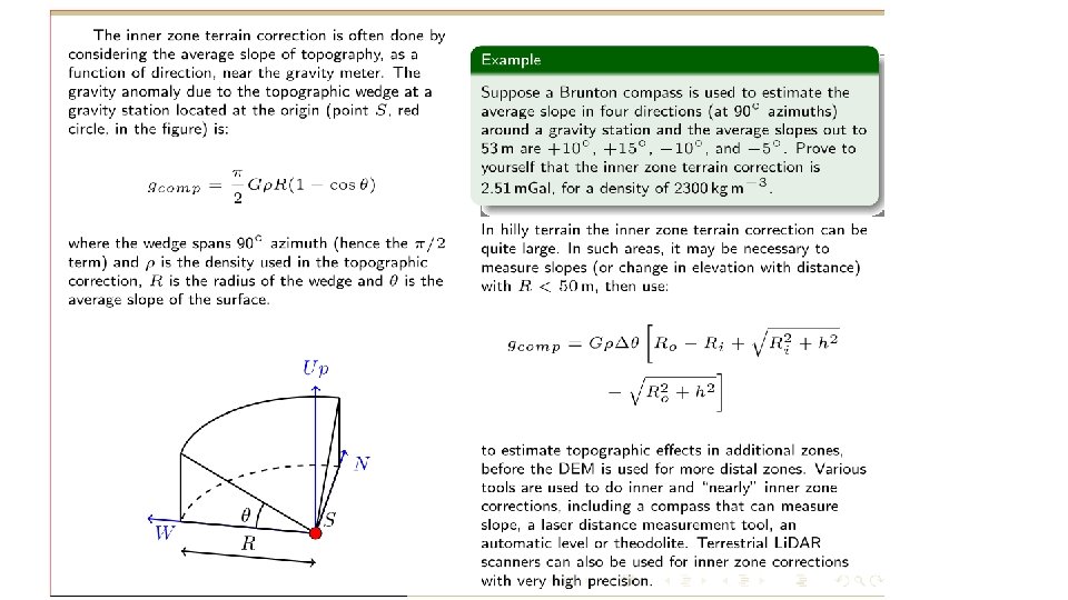
Terrain corrections • A correction applied to observed values obtained in geophysical surveys in order to remove the effect of variations in the observations due to the topography near observation sites.

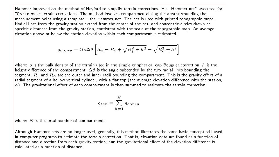
Apparently the terrain correction was first considered by Hayford and Bowie, around 1912, in interpreting gravity anomalies in the US. The problem of how to estimate the terrain correction was tackled by the geodesists Cassinis, Bullard, and Lambert in the 1930 s. Hammer developed a practical approach for performing terrain corrections out to about 22 km from the station. Bullard (1936) broke the topographic correction into three parts. The first two are the Bouguer correction (Bullard A), which approximates the topography to an infinite horizontal slab of thickness equal to the height of the station above the reference ellipsoid or another datum plane, and the curvature of the Earth (Bullard B) or spherical cap, which reduces the infinite Bouguer slab a spherical cap of the same thickness, with a surface radius of 166. 735 km approximately 1. 5 degree.

The Bullard B correction for the curvature of the Earth away from a gravity station GS : black is the section of the spherical cap directly underlying the infinite slab, which pulls downwards increasing the observed value of gravity