The Science of Macroeconomics Chapter 1 of Macroeconomics

The Science of Macroeconomics Chapter 1 of Macroeconomics, 10 th edition, by N. Gregory Mankiw ECO 62 Udayan Roy

What Macroeconomists Study • Why are some countries rich and others poor? • Why have some countries’ incomes grown rapidly over the past decade while others have stagnated? • Why do some countries have high rates of inflation while others maintain stable prices? • Why do all countries experience periods of economic stagnation or even crisis?

What Macroeconomists Study • What can government policy do to help an economy recover from a slump? • How do we know whether the amount of money that has been printed is too much, too little, or just enough? • Should China keep the value of the yuan fixed with respect to the US dollar? • Why has the US been running huge trade deficits? Does it matter?

Macroeconomics • Macroeconomics is the study of the economy as a whole • Macroeconomists collect data on incomes, price levels, interest rates, unemployment, and many other macroeconomic variables from different time periods and different countries • They then try to build general theories to explain the data that history gives them

Macroeconomics • My goal is to emphasize two aspects of macroeconomics that make it unique in the undergraduate curriculum: – The interconnections among the different parts of the economy are important – The dynamics that propel an economy forward over time are important

Macroeconomics: interconnections • First, macroeconomics is where students learn how to think about the economy as a collection of multiple markets that affect, and are affected by, each other. • It is not enough to analyze the goods market, and then the asset market, and then the labor market, and so on; all markets must be analyzed together, as interacting arenas of economic activity.

Macroeconomics: dynamics • Second, macroeconomics is where students learn to think dynamically about the economy. • It is important to understand how today leads to tomorrow, how tomorrow leads to the day after, and so on. • This emphasis on the dynamic laws of motion of an economy also makes macroeconomics different.

Macroeconomics • Macroeconomics is a young and imperfect science – Macroeconomists were not generally successful in predicting the global economic crisis of 2008 – Even after the crisis, they were unable to agree on what should be done to deal with the crisis • Nevertheless, the importance of the subject is clearer than ever

What sort of economic variables does macroeconomics try to explain? MACROECONOMIC DATA

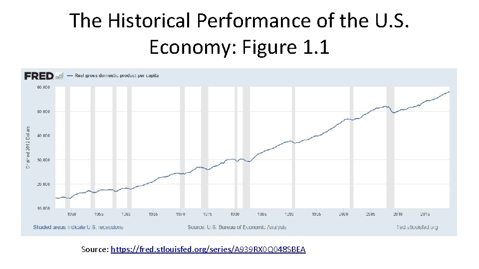
The Historical Performance of the U. S. Economy: Figure 1. 1 Source: https: //fred. stlouisfed. org/series/A 939 RX 0 Q 048 SBEA

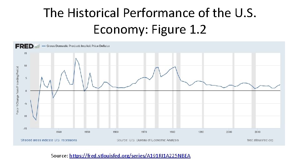
The Historical Performance of the U. S. Economy: Figure 1. 2 Source: https: //fred. stlouisfed. org/series/A 191 RI 1 A 225 NBEA

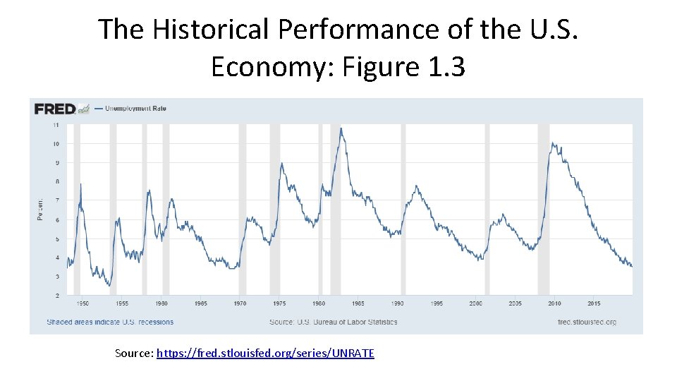
The Historical Performance of the U. S. Economy: Figure 1. 3 Source: https: //fred. stlouisfed. org/series/UNRATE

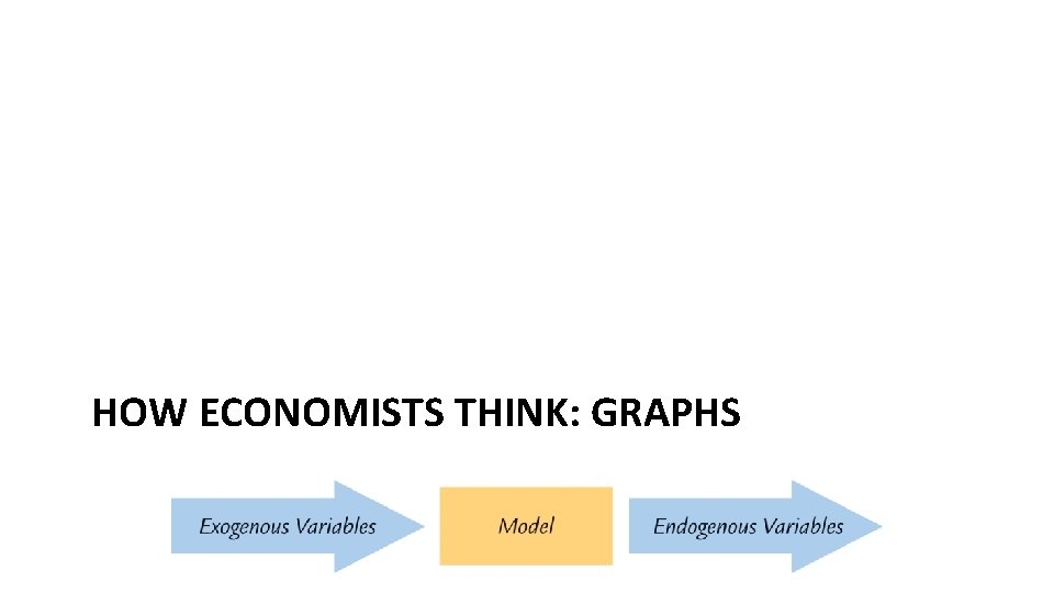
HOW ECONOMISTS THINK: GRAPHS

How Economists Think

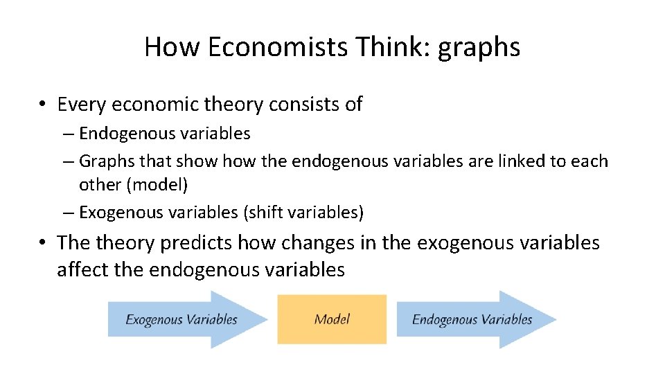
How Economists Think: graphs • Every economic theory consists of – Endogenous variables – Graphs that show the endogenous variables are linked to each other (model) – Exogenous variables (shift variables) • The theory predicts how changes in the exogenous variables affect the endogenous variables

Endogenous and exogenous variables • The endogenous variables of a theory are those variables whose fluctuations theory is trying to explain • The exogenous variables of a theory are those variables that theory assumes are crucial to understanding the endogenous variables, but are themselves not a concern of theory

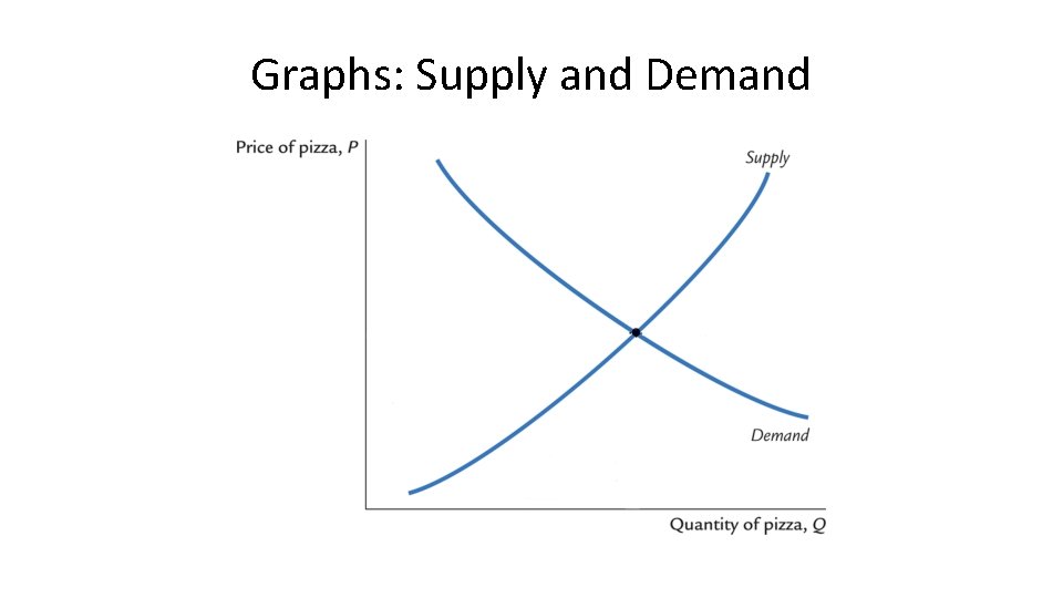
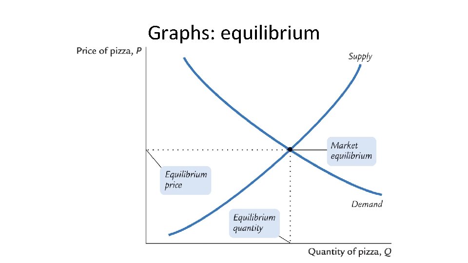
Graphs • Graphs are used to represent the various ways in which the endogenous variables are linked to each other • The graphs together determine the predicted values of the endogenous variables • Changes in exogenous variables cause the graphs to shift • The shifts of the graphs then tell us how the endogenous variables are likely to be affected

Example: the pizza market • Endogenous variables: price and quantity • The theory also needs – Graphs that show the endogenous variables are linked to each other (model) – Exogenous variables (shift variables)

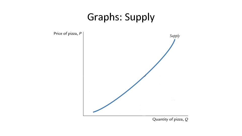
Graphs: Supply

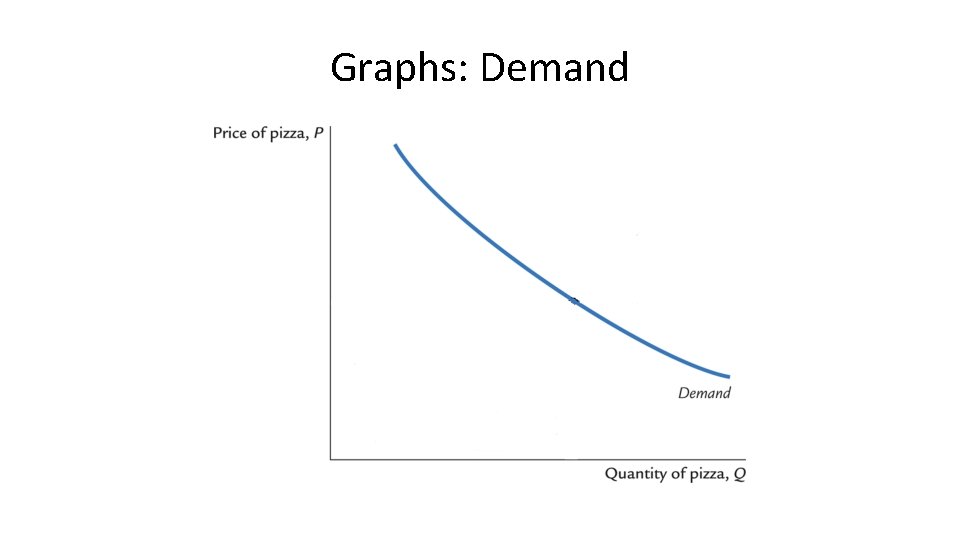
Graphs: Demand

Graphs: Supply and Demand

Graphs: equilibrium

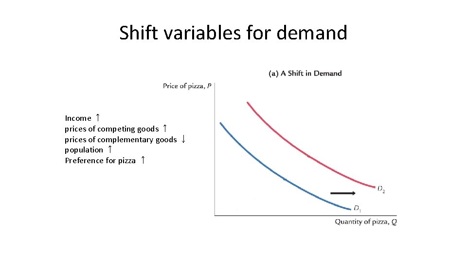
Shift variables for demand Income ↑ prices of competing goods ↑ prices of complementary goods ↓ population ↑ Preference for pizza ↑

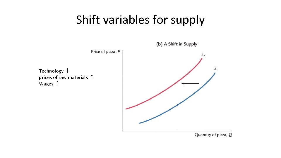
Shift variables for supply Technology ↓ prices of raw materials ↑ Wages ↑

Predictions • Now all our ducks are in a row! • We can use our theory to predict how changes in the exogenous (shift) variables will affect the endogenous variables

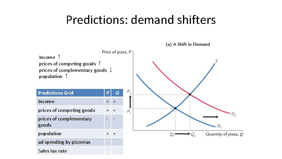
Predictions: demand shifters Income ↑ prices of competing goods ↑ prices of complementary goods ↓ population ↑ Predictions Grid P Income + + prices of competing goods + + prices of complementary goods - - population + + ad spending by pizzerias Sales tax rate Q

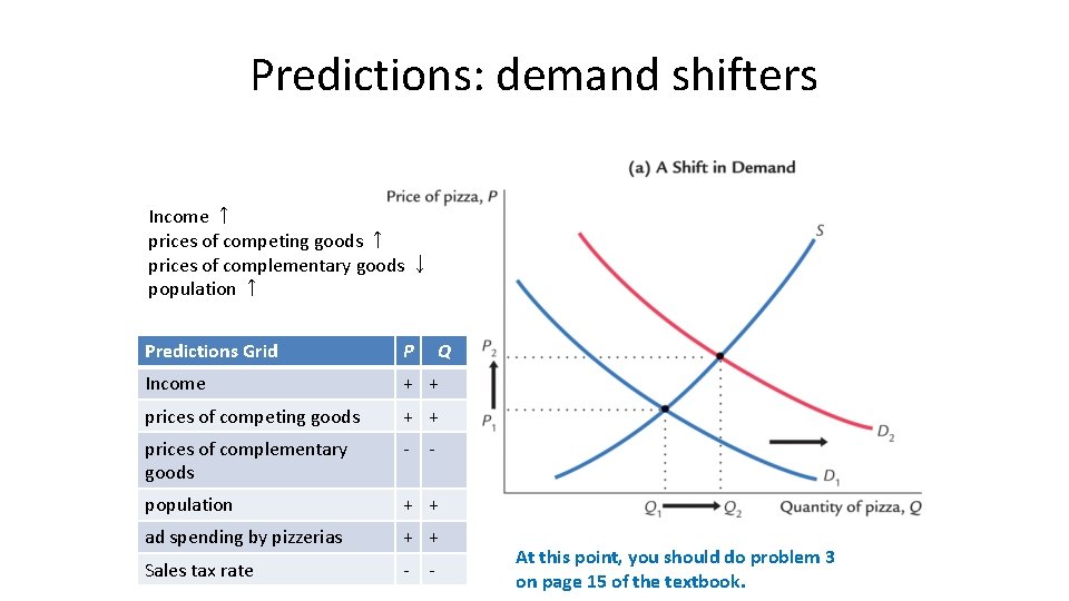
Predictions: demand shifters Income ↑ prices of competing goods ↑ prices of complementary goods ↓ population ↑ Predictions Grid P Q Income + + prices of competing goods + + prices of complementary goods - - population + + ad spending by pizzerias + + Sales tax rate - - At this point, you should do problem 3 on page 15 of the textbook.

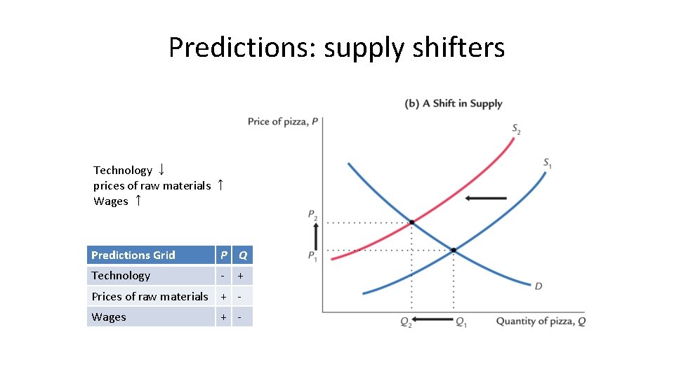
Predictions: supply shifters Technology ↓ prices of raw materials ↑ Wages ↑ Predictions Grid P Q Technology - + Prices of raw materials + Wages + -

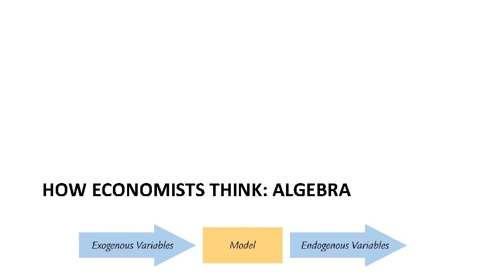
HOW ECONOMISTS THINK: ALGEBRA

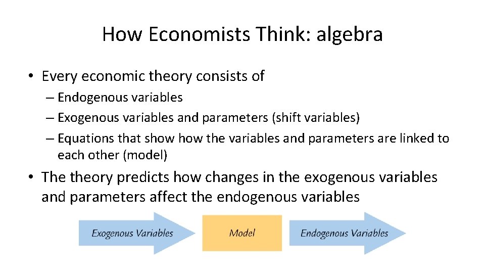
How Economists Think: algebra • Every economic theory consists of – Endogenous variables – Exogenous variables and parameters (shift variables) – Equations that show the variables and parameters are linked to each other (model) • The theory predicts how changes in the exogenous variables and parameters affect the endogenous variables

Equations • Each equation algebraically represents one idea/assumption about how the (endogenous and exogenous) variables and parameters are linked to each other

Solving the equations • If we have a set of equations such that the number of equations is equal to the number of endogenous variables in the equations, then we can usually solve the equations and express each endogenous variable in the equations in terms of the exogenous variables and parameters • These solutions predict the likely effects of the exogenous variables and parameters on the endogenous variables

Example: the pizza market • Endogenous variables: price (P), quantity demanded (Qd), and quantity supplied (Qs) • We still need – Exogenous variables and parameters – Equations linking all variables and parameters

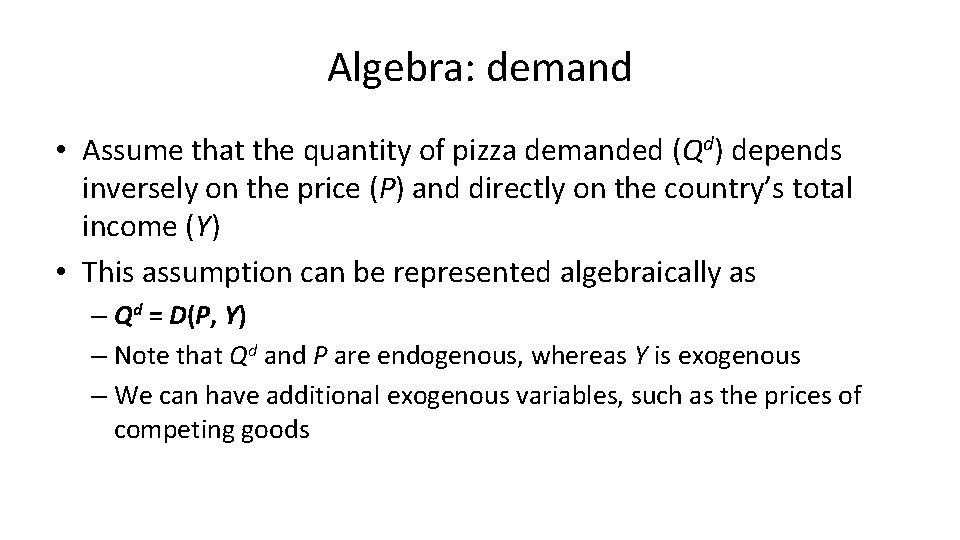
Algebra: demand • Assume that the quantity of pizza demanded (Qd) depends inversely on the price (P) and directly on the country’s total income (Y) • This assumption can be represented algebraically as – Qd = D(P, Y) – Note that Qd and P are endogenous, whereas Y is exogenous – We can have additional exogenous variables, such as the prices of competing goods

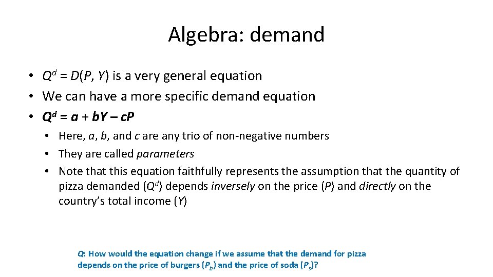
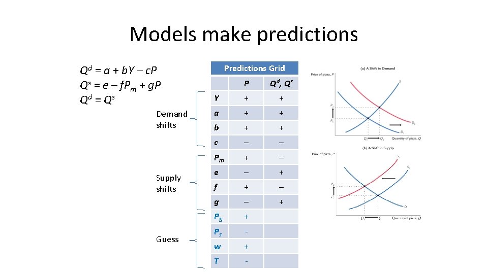
Algebra: demand • Qd = D(P, Y) is a very general equation • We can have a more specific demand equation • Qd = a + b. Y – c. P • Here, a, b, and c are any trio of non-negative numbers • They are called parameters • Note that this equation faithfully represents the assumption that the quantity of pizza demanded (Qd) depends inversely on the price (P) and directly on the country’s total income (Y) Q: How would the equation change if we assume that the demand for pizza depends on the price of burgers (Pb) and the price of soda (Ps)?

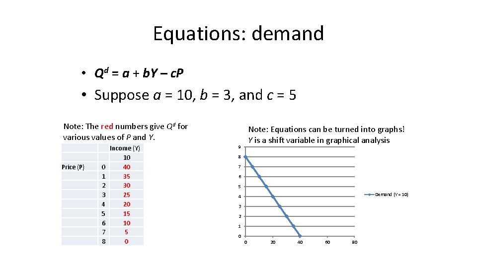
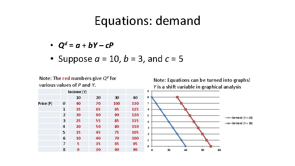
Equations: demand • Qd = a + b. Y – c. P • Suppose a = 10, b = 3, and c = 5 Note: The red numbers give Qd for various values of P and Y. Price (P) 0 1 2 3 4 5 6 7 8 Income (Y) 10 40 35 30 25 20 15 10 5 0 Note: Equations can be turned into graphs! Y is a shift variable in graphical analysis 9 8 7 6 5 Demand (Y = 10) 4 3 2 1 0 0 20 40 60 80

Equations: demand • Qd = a + b. Y – c. P • Suppose a = 10, b = 3, and c = 5 Note: The red numbers give Qd for various values of P and Y. Price (P) 0 1 2 3 4 5 6 7 8 Income (Y) 10 40 35 30 25 20 15 10 5 0 Note: Equations can be turned into graphs! Y is a shift variable in graphical analysis 9 20 70 65 60 55 50 45 40 35 30 30 100 95 90 85 80 75 70 65 60 40 130 125 120 115 110 105 100 95 90 8 7 6 5 Demand (Y = 10) 4 Demand (Y = 20) 3 2 1 0 0 20 40 60 80

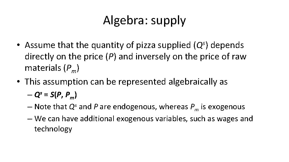
Algebra: supply • Assume that the quantity of pizza supplied (Qs) depends directly on the price (P) and inversely on the price of raw materials (Pm) • This assumption can be represented algebraically as – Qs = S(P, Pm) – Note that Qs and P are endogenous, whereas Pm is exogenous – We can have additional exogenous variables, such as wages and technology

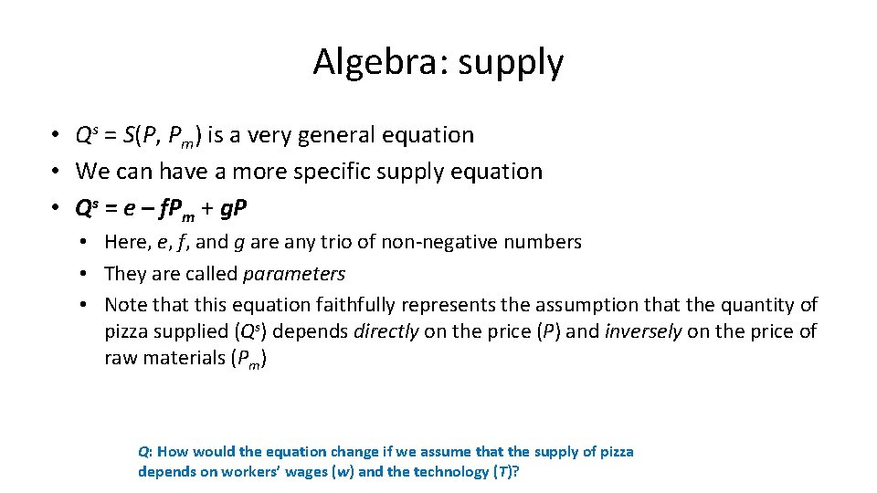
Algebra: supply • Qs = S(P, Pm) is a very general equation • We can have a more specific supply equation • Qs = e – f. Pm + g. P • Here, e, f, and g are any trio of non-negative numbers • They are called parameters • Note that this equation faithfully represents the assumption that the quantity of pizza supplied (Qs) depends directly on the price (P) and inversely on the price of raw materials (Pm) Q: How would the equation change if we assume that the supply of pizza depends on workers’ wages (w) and the technology (T)?

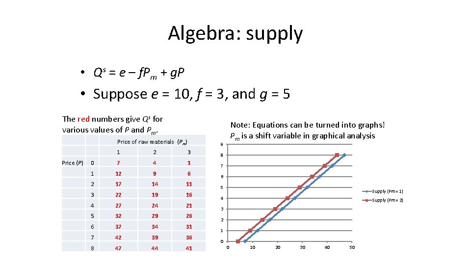
Algebra: supply • Qs = e – f. Pm + g. P • Suppose e = 10, f = 3, and g = 5 The red numbers give Qs for various values of P and Pm. Price (P) Price of raw materials (Pm) 9 1 2 3 8 0 7 4 1 7 1 12 9 6 6 2 17 14 11 5 3 22 19 16 4 27 24 21 5 32 29 26 6 37 34 31 7 42 39 36 8 47 44 41 Note: Equations can be turned into graphs! Pm is a shift variable in graphical analysis Supply (Pm = 1) 4 Supply (Pm = 2) 3 2 1 0 0 10 20 30 40 50

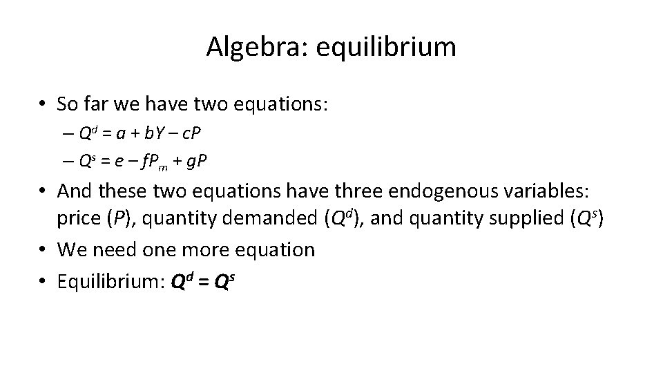
Algebra: equilibrium • So far we have two equations: – Qd = a + b. Y – c. P – Qs = e – f. Pm + g. P • And these two equations have three endogenous variables: price (P), quantity demanded (Qd), and quantity supplied (Qs) • We need one more equation • Equilibrium: Qd = Qs

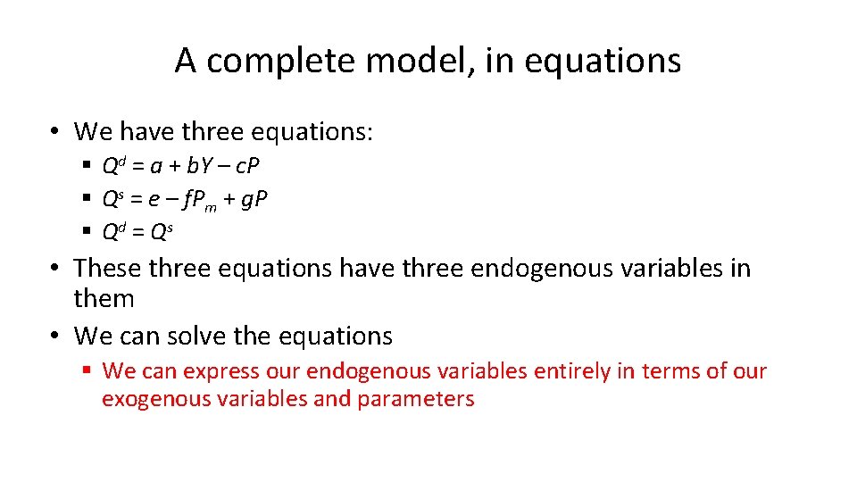
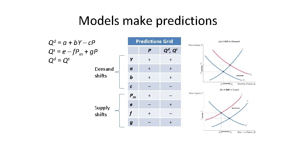
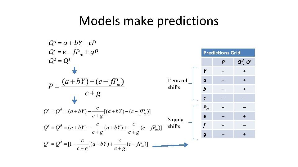
A complete model, in equations • We have three equations: § Qd = a + b. Y – c. P § Qs = e – f. Pm + g. P § Qd = Qs • These three equations have three endogenous variables in them • We can solve the equations § We can express our endogenous variables entirely in terms of our exogenous variables and parameters

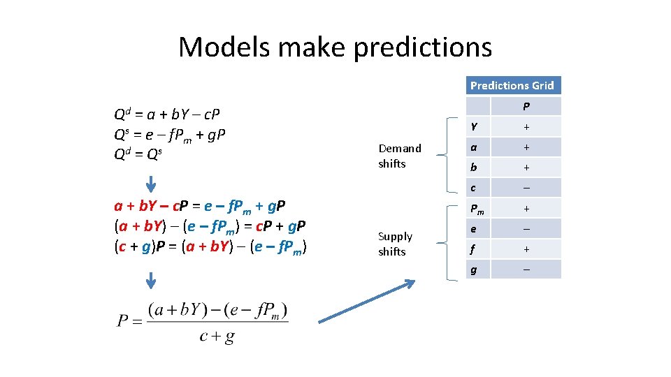
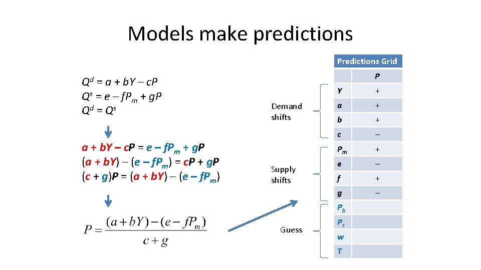
Models make predictions Predictions Grid Qd = a + b. Y – c. P Qs = e – f. Pm + g. P Qd = Qs a + b. Y – c. P = e – f. Pm + g. P (a + b. Y) – (e – f. Pm) = c. P + g. P (c + g)P = (a + b. Y) – (e – f. Pm) P Demand shifts Supply shifts Y + a + b + c – Pm + e – f + g –

Models make predictions Predictions Grid Qd = a + b. Y – c. P Qs = e – f. Pm + g. P Qd = Qs a + b. Y – c. P = e – f. Pm + g. P (a + b. Y) – (e – f. Pm) = c. P + g. P (c + g)P = (a + b. Y) – (e – f. Pm) P Demand shifts Supply shifts Y + a + b + c – Pm + e – f + g – Pb Guess Ps w T

Models make predictions Predictions Grid Qd = a + b. Y – c. P Qs = e – f. Pm + g. P Qd = Qs a + b. Y – c. P = e – f. Pm + g. P (a + b. Y) – (e – f. Pm) = c. P + g. P (c + g)P = (a + b. Y) – (e – f. Pm) P Demand shifts Supply shifts Guess Y + a + b + c – Pm + e – f + g – Pb + Ps - w + T -

Models make predictions Qd = a + b. Y – c. P Qs = e – f. Pm + g. P Qd = Qs Demand shifts Supply shifts Predictions Grid P Qd, Qs Y + + a + + b + + c – – Pm + – e – + f + – g – +

Models make predictions Qd = a + b. Y – c. P Qs = e – f. Pm + g. P Qd = Qs Demand shifts Supply shifts Guess Predictions Grid P Qd, Qs Y + + a + + b + + c – – Pm + – e – + f + – g – + Pb + Ps - w + T -

Models make predictions Qd = a + b. Y – c. P Qs = e – f. Pm + g. P Qd = Qs Demand shifts Supply shifts Guess Predictions Grid P Qd, Qs Y + + a + + b + + c – – Pm + – e – + f + – g – + Pb + + Ps - - w + - T - +

Models make predictions Qd = a + b. Y – c. P Qs = e – f. Pm + g. P Qd = Qs Predictions Grid Demand shifts Supply shifts P Qd, Qs Y + + a + + b + + c – – Pm + – e – + f + – g – +

The end of the line • Exogenous variables and parameters are, by definition, not the concern of theory • Therefore, once all endogenous variables have been expressed entirely in terms of exogenous variables and parameters, our job is done • We can’t say anything more • All that remains is to use data to test whether the predictions are true in the real world

Onward • In the rest of this course we will use the graphical and algebraic techniques of this chapter to analyze all sorts of macroeconomic problems