SIMPLE LINEAR REGRESSION Causality also referred to cause

SIMPLE LINEAR REGRESSION

Causality (also referred to 'cause and effect') is the relation between one process (the cause) and another (the effect), where the first is understood to be partly responsible for the second. In general, a process has many causes, which are said to be causal factors for it, and all lie in its past. An effect can in turn be a cause of many other effects, which all lie in its future.

Cause Effect Reason Result Indepent Dependent

Some causality questions 1. Does the advertising (C) will increase sales (E)? 2. Is there a causal relationship between the number of people who pass in front of a store and the sale of the store? 3. Does personal income determine food consumption?

X Independent Y Dependent Ads Sale Cause Effect Reason Result

X Independent Ads Y Dependent Sale Profit Cause Effect Reason Result

Interaction Variables Effect Inflation Rate Cause Exchange Rate Effect

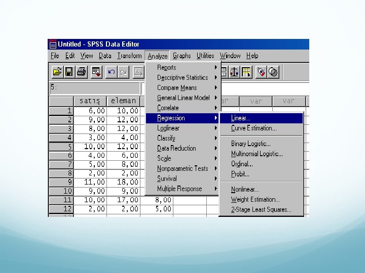
Regression Types

Dynamic Regression The time series models in the previous two chapters allow for the inclusion of information from the past observations of a series, but not for the inclusion of other information that may be relevant.

Years Ads Expenditure Sales TL 2005 1000 10. 000 2006 2000 2007 3000 30. 000 2008 2000 25. 000 2009 2000 30. 000 2010 1700 20. 000

Static Regression Casual relation between two variable in a fixed time period

The adv expenditures and sales of 5 firms in 2014 Names of firms Adv Expenditures Sales TL 1 2000 10. 000 2 3000 15. 000 3 20. 000 50. 000 4 3000 5 25. 000 50. 000

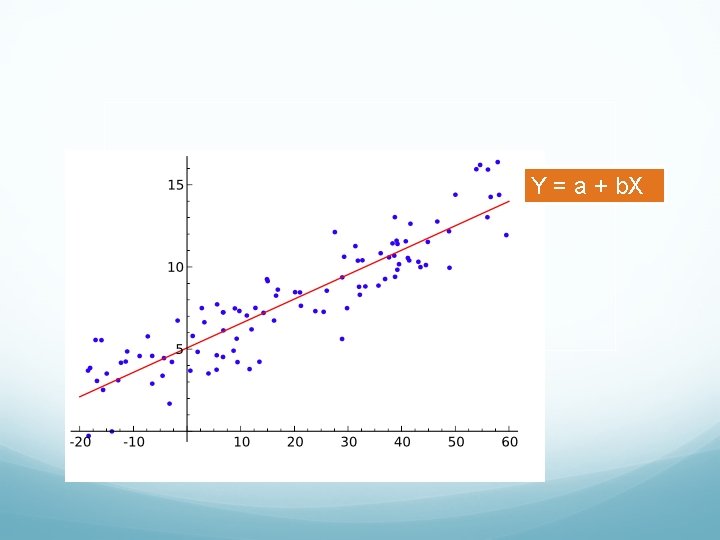
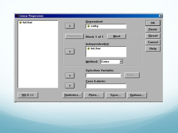
Simple Linear Regression

In Simple linear regression is the least squares estimator of a linear regression model with a single (independent) variable. In other words, simple linear regression fits a straight line through the set of n points in such a way that makes the sum of squared residuals of the model (that is, vertical distances between the points of the data set and the fitted line) as small as possible. The adjective simple refers to the fact that the outcome variable is related to a single predictor. The slope of the fitted line is equal to the correlation between y and x corrected by the ratio of standard deviations of these variables. The intercept of the fitted line is such that it passes through the center of mass (x, y) of the data points.

These questions can be asked by regression

1. Is there an association between independent variables and the dependent variable? 2. Does the independent variable(s) explain the variation in dependent variable? 3. Is the causal relation between the independent variable(s) and dependent variable linear or non linear? 4. In dynamic regression can we make any estimation for the future?

Formulation of Simple linear Regression Model Y = f(X) = 0 + 1 Xi+ i

Example: A firm wonders the casual relation between its yearly advertisement expenditures and annual sales.

Table 1 Advs Expenditures and sales of a Firm Observations Advs Expenditures Million TL Sales Million TL

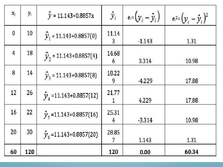
The Calculation of Linear Regression Model = 10 = 20

Deductions from the model

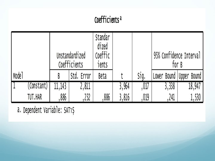
1. If the firm makes no advs X=0, the sale will be 11 Million 143 thousands TL. 2. Because the parameter b shows the tendency, it can be deduct that if the firm increases its adv one unit (million), the sales will increase 0. 8857 Million or 885. 7 Thousands TL. Is it profitable to make adv. ?

3. Because the sign of b is positive, it can be said that the more the adv increases, the more the sale will increase. 4. If we spent 18 million TL for adv, the sale will be y=11. 143+0. 8857(18)=11. 159 which is not logic to make this adv. 5. If we want to increase the sale to 25 million TL, we should make 15. 645 million TL adv. 25=11. 143+0. 8857 X, X=15. 645 TL

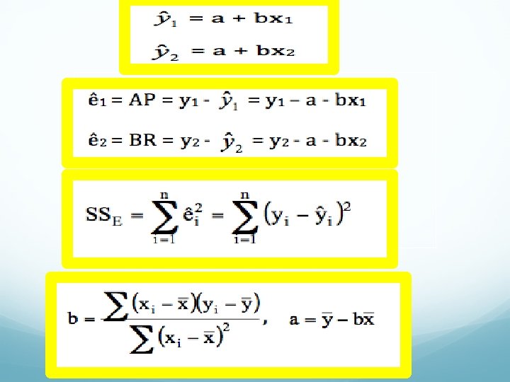
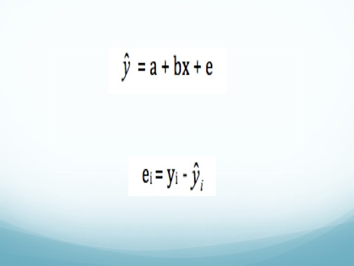
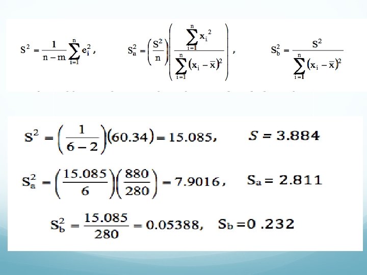
The outcomes should be tested statistically How to calculate error terms of a regression model?

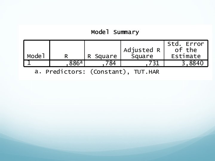
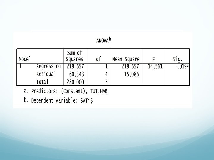
Determination coefficient and Testing The Regression Model

SST: Total Sum of Square SSR: Regression Sum of Square SSE: Error Sum of Square Formula to calculate SSR and SSE

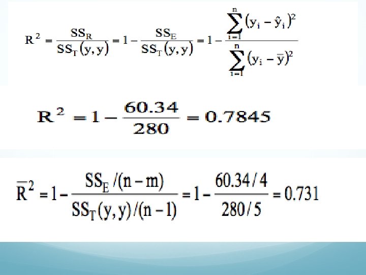
Determination coefficient shows how much the independent variable(s) explain the variation in dependent variable.

With 0. 05 significance level and 1 to 4 df the table value is 7. 71. Because the calculated value is bigger than 7. 71 it can be said that the whole model is valid.

Testing The Coefficients

Because this test double tailed the t values for a and b can be calculated

This is a double tailed t test so significance level is 0. 05/2= 0. 025. The df is n-2=6 -2=4. The table value is 2. 77. Both calculated t value of the coefficients are bigger than the table value. Therefore H 0 will be rejected and H 1 will be accepted. This means that the values of the parameters a and b are different than the zero. In this case the regression model is valid and can be interpreted.

Multiple Regression

Some questions answered by multiple regression 1. Can the variation in the sale be explained by adv. expenditures, prices, distribution levels at the same time? 2. Is there any casualty relation between market shares one the one hand adv. Expenditures, sales promotion budgets on the other hand? 3. Can consumer quality perceptions be determined by price perceptions, brand image and brand features?

Y = 0 + 1 X 1+ 2 X 2+ 3 X 3+. . . + k Xk + y = a + b 1 x 1 + b 2 x 2 + b 3 x 3 +. . . + bkxk

Multiple regression can not be used: 1. If the number of the variables are more than the number of the observations. 2. If The correlations among the independent variables are strong

Y = (x’x)1 x’y

Application of Multiple Regression Analysis

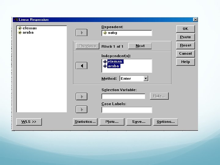
Example A firm has 12 different sales regions. Sales, the number of the salesmen and sales cars are shown in the table. Is there any causal relation among the variables?

Nu of Cars Monthly Sales Million TL (Milyar Aylık Satışlar Nu of Salesmen Eleman Sayısı TL) (Y) (X 1) Araba Sayısı (X 2) 1 6 10 3 2 9 12 11 3 8 12 4 4 3 4 1 5 10 12 11 6 4 6 1 7 5 8 7 8 2 2 4 9 11 18 8 10 9 9 10 11 10 17 8 12 2 2 5 Bölgeler Regions

Correlation Coefficients Correlation Adjusted Standard Error Result Of Variance analysis Degree of Freedom Sum of Squares Regression Residuals F Value Significance level

Regression. Findings Regression Equation Variables Coefficients Standard Errors Fixed Value Regression Equation Standardized Coefficients Significance

Conclusion and Interpretation of the Equation

1. Let’s assume that we need to open a new region and 15 Salesmen and 6 cars will be used in this region. Can we estimate the sales of this region? y= 0. 337 + 0. 481(15) + 0. 289(6) = 9. 29 Million TL 2. Provided that the number of cars remain constant, a new member taken to any region, will increase the monthly sales 0. 481 Million TL or 481. 000 TL. 3. Provided that the number of salesmen remain constant, a new car added to any region, will increase the monthly sales 0. 289 Million TL or 289. 000 TL

Both two independent variables have positive sign. This means that the relation between each independent variables and the dependent variable is positive. As the nu of salesmen increases so does total sales. 4. 5. The total model is significant at the level of 0. 00 and with F value 77. 29. So according the determination oefficient R 2 shows that 93% of the variation in the total sale can be explained by salesmen and car numbers. 6. Since the significance of t values for X 1 and X 2 which are 0. 00 and 0. 009 these variable are two different causes which affect total sale. Also because the t value of X 1 (8. 16) is bigger than the t value of X 2 (3. 35), X 1 explains the variation in total sale better than X 2

Using Dummy Variable

1. Nonmetric with two parts: male/female 2. Nonmetric with more than two parts: Education levels, occupations, consumption frequency of any products

In order to change the nonmetric scales to metric, 1 -0 technic could be used

İf male is 1 the female will be 0 or if married people is 1 the unmarried people will be 0 Different technic should be used if there are more than two choices

Kullanma Usage Rate of a. Sıklığı product Normal Coding Kukla Değişkenler Dummy Variables Kodlama Normal Coding X 1 X 2 X 3 Hiç kullanmayanlar Nonusers 1 1 0 0 Az kullananlar Light users 2 0 1 0 Orta kullananlar Normal users 3 0 0 1 Çok kullananlar Heavy users 4 0 0 0

Let’s assume that we are employing 12 salesmen. Their education levels are shown below. I education levels affect sales volume? Assume that elementary school 1, middle school 2, high school 3 and faculty 4

Regions Bölgeler 1 2 3 4 5 6 7 8 9 10 11 12 Aylık Satışlar Monthly Sales (Milyar Million TL TL) 6 9 8 3 10 4 5 2 11 9 10 2 Education Levels Eğitim Düzeyi Faculty 4 (Fakülte) 2 (Ortaokul) Middle School 2 (Ortaokul) 4 (Fakülte) Faculty 2 (Ortaokul) Middle School 3 High (Lise)School Elementary School 1 (İlkokul) High School 3 (Lise) 4 (Fakülte) Faculty 1 Elementary (İlkokul) School

Kullanma Usage Rate of a. Sıklığı product Normal Coding Kukla Değişkenler Dummy Variables Kodlama Normal Coding X 1 X 2 X 3 Hiç kullanmayanlar Nonusers 1 1 0 0 Az kullananlar Light users 2 0 1 0 Orta kullananlar Normal users 3 0 0 1 Çok kullananlar Heavy users 4 0 0 0

Eğitim Düzeyleri 1 2 3 4 5 6 7 8 9 10 11 12 Aylık Satışlar (Milyar TL) 6 9 8 3 10 4 5 2 11 9 10 2 Eğitim Düzeyi 4 (Fakülte) 2(Ortaokul) 3 (Lise) 1 (İlkokul) 3 (Lise) 4 (Fakülte) 1 (İlkokul) X 1 X 2 X 3 0 0 0 0 1 1 0 0 0 0 1 1 0 0

Standartlaştırılmamış ştırılmış Katsayılar Sum of Means Model 1 Squares DF Standard Regression B 77, 500 Error Model 3 (Fixed v. ) 1 8, 750 1, 165 Square Beta 25, 833 Residuals x 1 43, 417 -6, 750 T Signific Signi F ance Value nican s , 035 ce 4, 760 7, 512 , 000 8 2, 018 5, 427 -, 792 -3, 346 , 010 x 2 Total -3, 750 1, 779 -, 512 -2, 108 , 068 x 3 1, 779 -, 057 -, 234 , 821 120, 917 -, 417 11 Because the significance of t values for X 2 and X 3 are above 0. 05 these two variables has no causal effect on the sales. Only the significance of X 1 is valid son we can interpret only this variable

1. Because the sign of X 1 is negative, there is a negative correlation between X 1 and sales. As education level progresses from 1 (elementary school) to 0 (other levels), the sales rise. Actually progressing the education level from 1 to 0 is not an increase but decrease 0 indicates middle, high and undergraduate school. 2. So while education level increases from 1 to 0 the sales are increasing respectively 3. As education level increase one unite from elementary school to the other levels, the aes will increase 6 million and 759. 000 TL

Problem of Multicolinearity

In order to arise the explanation rate, some times we need to add a new independent variable to the regression model. This addition may decrease the effectiveness the exist independent variables, because of increasing the correlation between the variables. This addition also reduce t value. This is a kind of statistical disease because the high coloration between the new independent variable and the others independent variables, will reduce the effectiveness of the whole independent variables. So we need to eliminate some of the independent variables.

Nu of Cars Monthly Sales Million TL (Milyar Aylık Satışlar Nu of Salesmen Eleman Sayısı TL) (Y) (X 1) Araba Sayısı (X 2) 1 6 10 3 2 9 12 11 3 8 12 4 4 3 4 1 5 10 12 11 6 4 6 1 7 5 8 7 8 2 2 4 9 11 18 8 10 9 9 10 11 10 17 8 12 2 2 5 Bölgeler Regions

Regression Analysis Regression Model Regression Results Variables Coefficients Standard Errors Fixed Value Regression Equation Standardized Coefficients Significance

Coefficients Fixed Value Standardized Coefficients Significa nce

Let us see the correlation coefficients among the variables

Total Celeries X 3 Maaş Nu Car Araba X 2 Salesmen Eleman X 1 1. 000 0. 639 -0. 999 Nu Cars X 2 Araba 0. 639 1. 000 -0. 659 Salesmen X 1 Eleman -0. 999 -0. 659 1. 000 It is clear that the correlation between X 3 and other variables are very high. So this is the reason of multicollinearity.

Stepwise Regression

The End