Programme 13 Curves and curve fitting PROGRAMME 13

Programme 13: Curves and curve fitting PROGRAMME 13 CURVES AND CURVE FITTING STROUD Worked examples and exercises are in the text

Programme 13: Curves and curve fitting Introduction Standard curves Asymptotes Systematic curve sketching, given the equation of the curve Curve fitting Method of least squares Correlation STROUD Worked examples and exercises are in the text

Programme 13: Curves and curve fitting Introduction Standard curves Asymptotes Systematic curve sketching, given the equation of the curve Curve fitting Method of least squares Correlation STROUD Worked examples and exercises are in the text

Programme 13: Curves and curve fitting Introduction The purpose of this Programme is to develop methods for establishing the relationship between two variables whose values have been obtained by experiment. Before doing this it is necessary to consider the algebraic relationships that give rise to standard geometric shapes. STROUD Worked examples and exercises are in the text

Programme 13: Curves and curve fitting Introduction Standard curves Asymptotes Systematic curve sketching, given the equation of the curve Curve fitting Method of least squares Correlation STROUD Worked examples and exercises are in the text

Programme 13: Curves and curve fitting Introduction Standard curves Asymptotes Systematic curve sketching, given the equation of the curve Curve fitting Method of least squares Correlation STROUD Worked examples and exercises are in the text

Programme 13: Curves and curve fitting Standard curves Straight line Second-degree curves Third-degree curves Circle Ellipse Hyperbola Logarithmic curves Exponential curves Hyperbolic curves Trigonometrical curves STROUD Worked examples and exercises are in the text

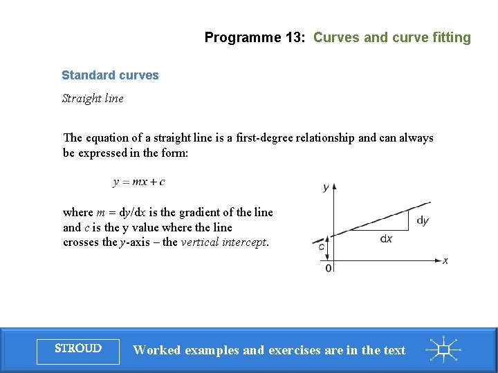
Programme 13: Curves and curve fitting Standard curves Straight line The equation of a straight line is a first-degree relationship and can always be expressed in the form: where m = dy/dx is the gradient of the line and c is the y value where the line crosses the y-axis – the vertical intercept. STROUD Worked examples and exercises are in the text

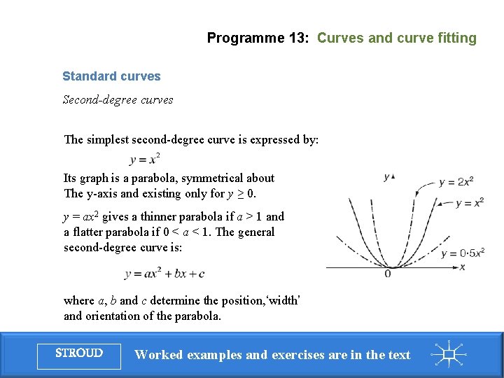
Programme 13: Curves and curve fitting Standard curves Second-degree curves The simplest second-degree curve is expressed by: Its graph is a parabola, symmetrical about The y-axis and existing only for y ≥ 0. y = ax 2 gives a thinner parabola if a > 1 and a flatter parabola if 0 < a < 1. The general second-degree curve is: where a, b and c determine the position, ‘width’ and orientation of the parabola. STROUD Worked examples and exercises are in the text

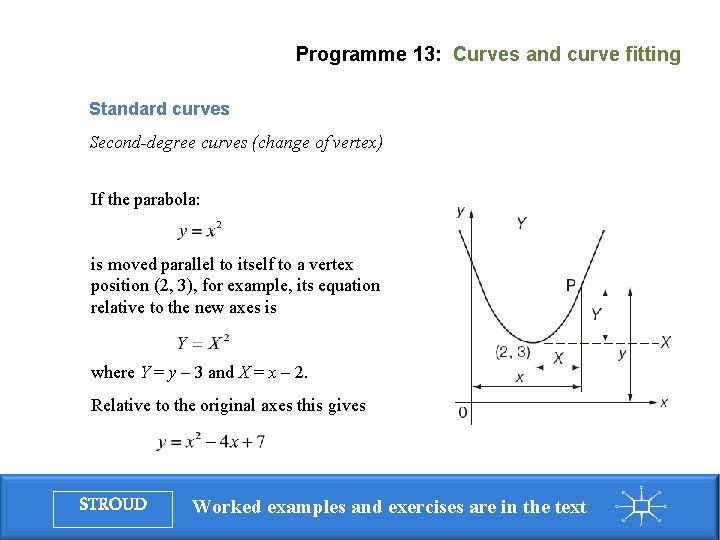
Programme 13: Curves and curve fitting Standard curves Second-degree curves (change of vertex) If the parabola: is moved parallel to itself to a vertex position (2, 3), for example, its equation relative to the new axes is where Y = y – 3 and X = x – 2. Relative to the original axes this gives STROUD Worked examples and exercises are in the text

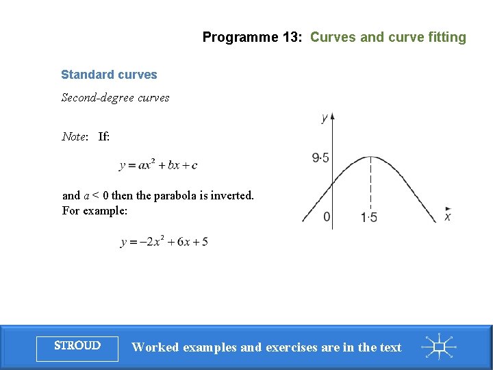
Programme 13: Curves and curve fitting Standard curves Second-degree curves Note: If: and a < 0 then the parabola is inverted. For example: STROUD Worked examples and exercises are in the text

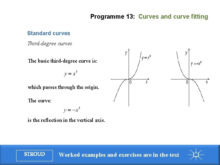
Programme 13: Curves and curve fitting Standard curves Third-degree curves The basic third-degree curve is: which passes through the origin. The curve: is the reflection in the vertical axis. STROUD Worked examples and exercises are in the text

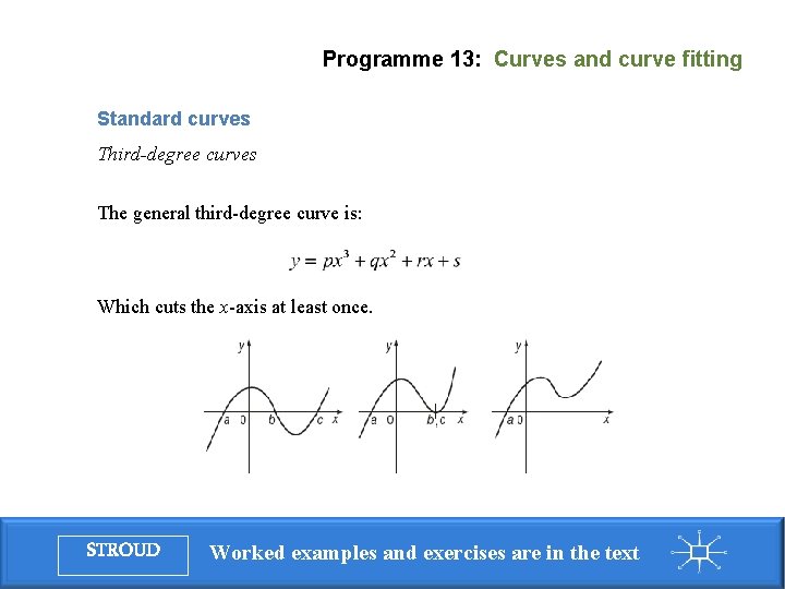
Programme 13: Curves and curve fitting Standard curves Third-degree curves The general third-degree curve is: Which cuts the x-axis at least once. STROUD Worked examples and exercises are in the text

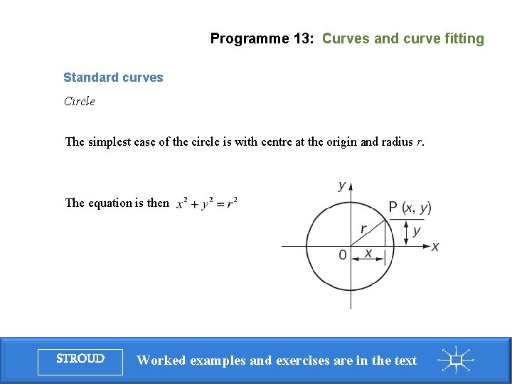
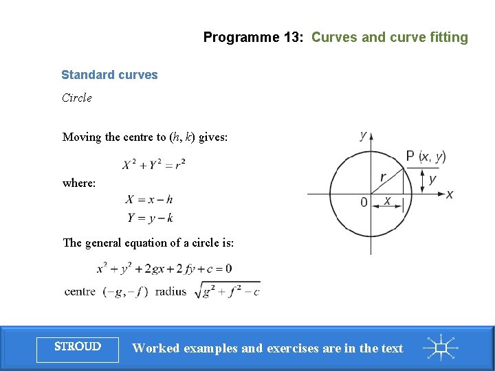
Programme 13: Curves and curve fitting Standard curves Circle The simplest case of the circle is with centre at the origin and radius r. The equation is then STROUD Worked examples and exercises are in the text

Programme 13: Curves and curve fitting Standard curves Circle Moving the centre to (h, k) gives: where: The general equation of a circle is: STROUD Worked examples and exercises are in the text

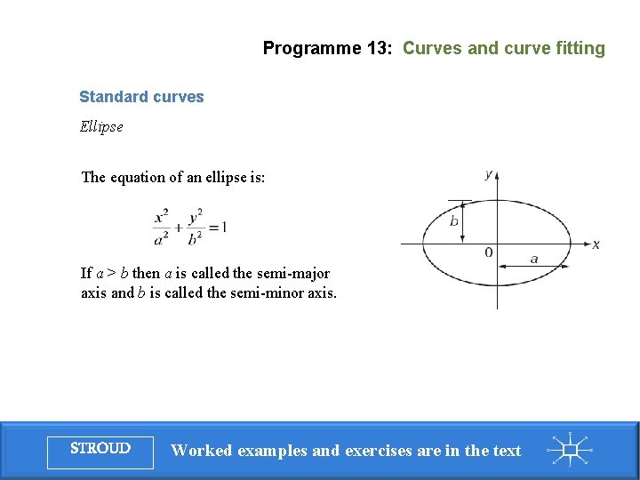
Programme 13: Curves and curve fitting Standard curves Ellipse The equation of an ellipse is: If a > b then a is called the semi-major axis and b is called the semi-minor axis. STROUD Worked examples and exercises are in the text

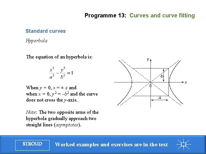
Programme 13: Curves and curve fitting Standard curves Hyperbola The equation of an hyperbola is: When y = 0, x = ± a and when x = 0, y 2 = –b 2 and the curve does not cross the y-axis. Note: The two opposite arms of the hyperbola gradually approach two straight lines (asymptotes). STROUD Worked examples and exercises are in the text

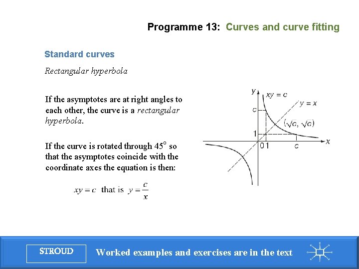
Programme 13: Curves and curve fitting Standard curves Rectangular hyperbola If the asymptotes are at right angles to each other, the curve is a rectangular hyperbola. If the curve is rotated through 45 o so that the asymptotes coincide with the coordinate axes the equation is then: STROUD Worked examples and exercises are in the text

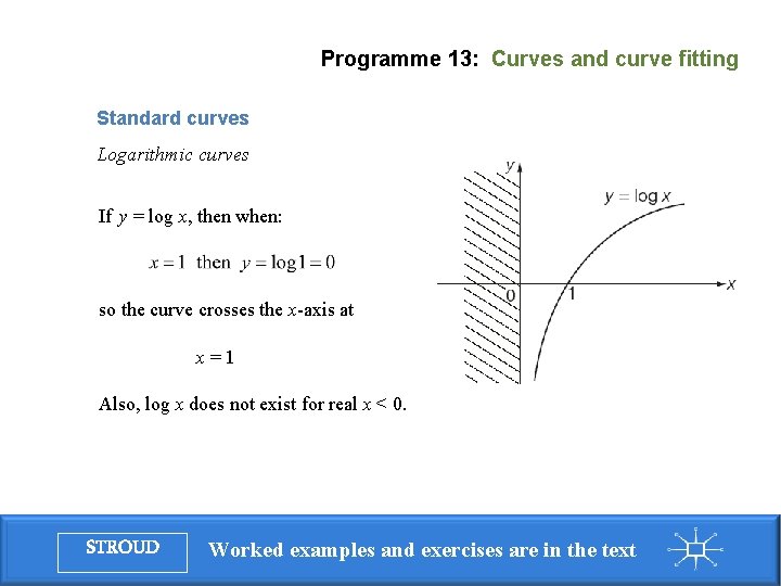
Programme 13: Curves and curve fitting Standard curves Logarithmic curves If y = log x, then when: so the curve crosses the x-axis at x=1 Also, log x does not exist for real x < 0. STROUD Worked examples and exercises are in the text

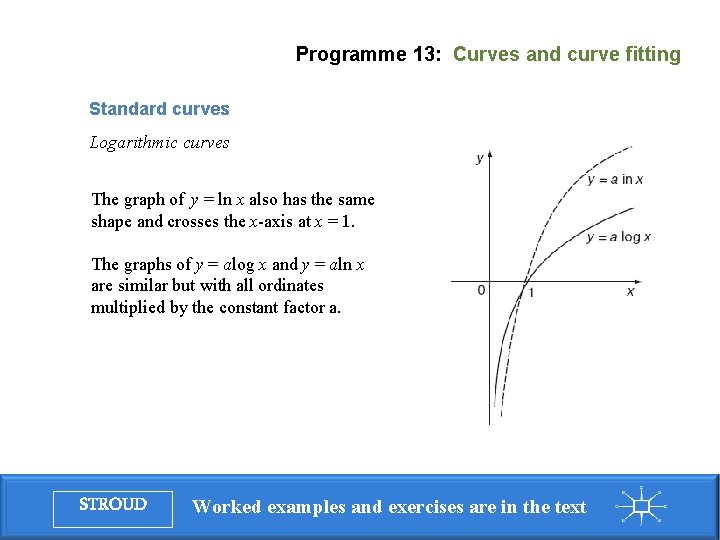
Programme 13: Curves and curve fitting Standard curves Logarithmic curves The graph of y = ln x also has the same shape and crosses the x-axis at x = 1. The graphs of y = alog x and y = aln x are similar but with all ordinates multiplied by the constant factor a. STROUD Worked examples and exercises are in the text

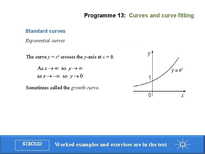
Programme 13: Curves and curve fitting Standard curves Exponential curves The curve y = ex crosses the y-axis at x = 0. Sometimes called the growth curve. STROUD Worked examples and exercises are in the text

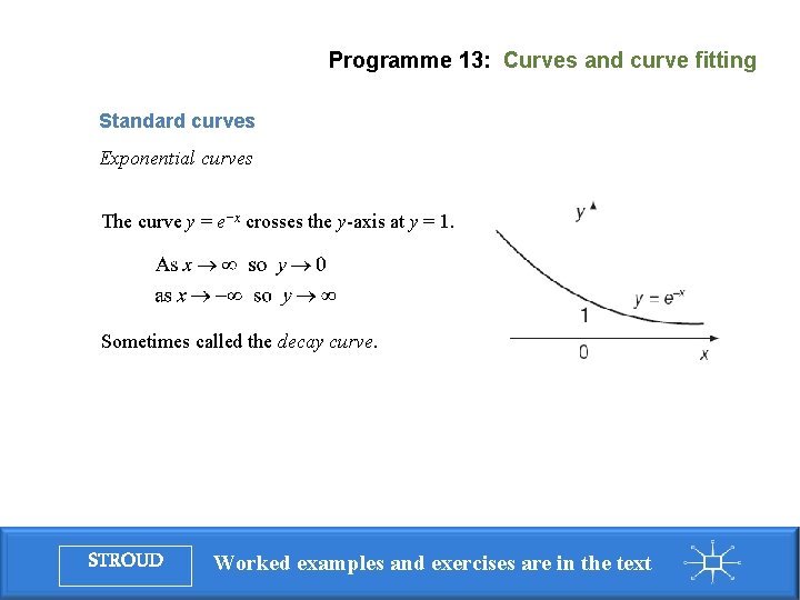
Programme 13: Curves and curve fitting Standard curves Exponential curves The curve y = e−x crosses the y-axis at y = 1. Sometimes called the decay curve. STROUD Worked examples and exercises are in the text

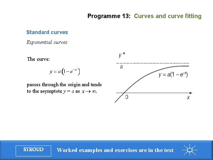
Programme 13: Curves and curve fitting Standard curves Exponential curves The curve: passes through the origin and tends to the asymptote y = a as. STROUD Worked examples and exercises are in the text

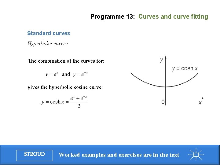
Programme 13: Curves and curve fitting Standard curves Hyperbolic curves The combination of the curves for: gives the hyperbolic cosine curve: STROUD Worked examples and exercises are in the text

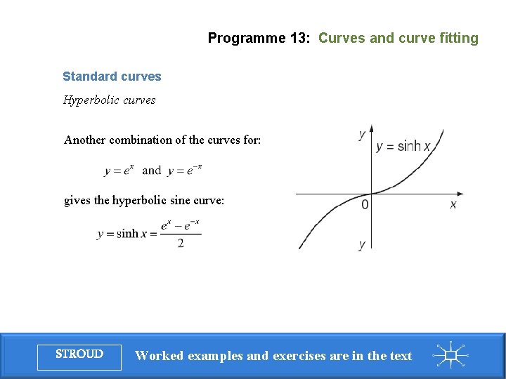
Programme 13: Curves and curve fitting Standard curves Hyperbolic curves Another combination of the curves for: gives the hyperbolic sine curve: STROUD Worked examples and exercises are in the text

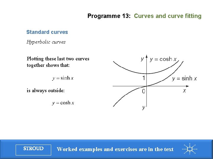
Programme 13: Curves and curve fitting Standard curves Hyperbolic curves Plotting these last two curves together shows that: is always outside: STROUD Worked examples and exercises are in the text

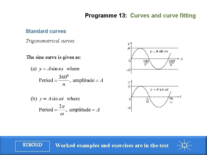
Programme 13: Curves and curve fitting Standard curves Trigonometrical curves The sine curve is given as: STROUD Worked examples and exercises are in the text

Programme 13: Curves and curve fitting Introduction Standard curves Asymptotes Systematic curve sketching, given the equation of the curve Curve fitting Method of least squares Correlation STROUD Worked examples and exercises are in the text

Programme 13: Curves and curve fitting Introduction Standard curves Asymptotes Systematic curve sketching, given the equation of the curve Curve fitting Method of least squares Correlation STROUD Worked examples and exercises are in the text

Programme 13: Curves and curve fitting Asymptotes Determination of an asymptote Asymptotes parallel to the x- and y-axes STROUD Worked examples and exercises are in the text

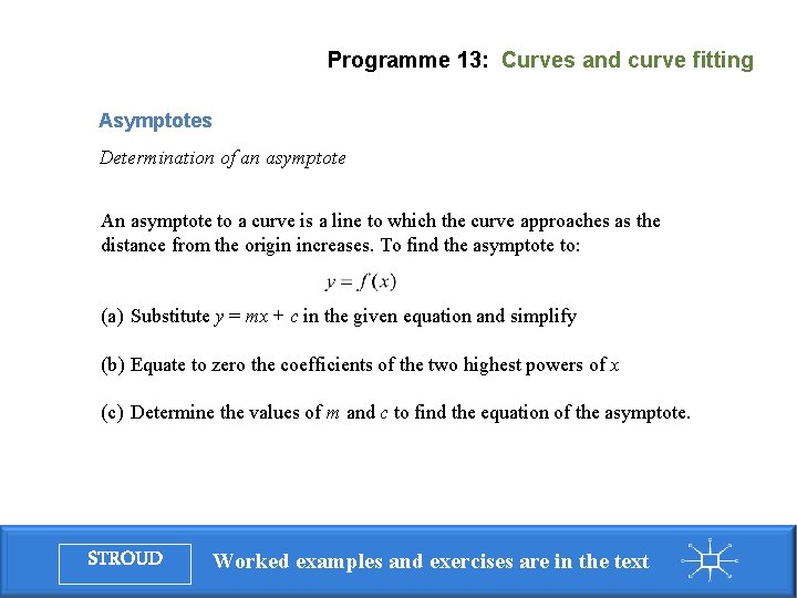
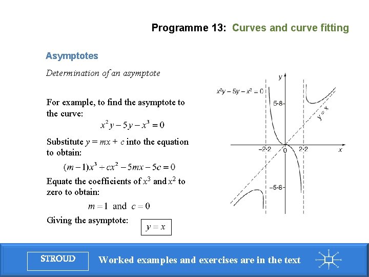
Programme 13: Curves and curve fitting Asymptotes Determination of an asymptote An asymptote to a curve is a line to which the curve approaches as the distance from the origin increases. To find the asymptote to: (a) Substitute y = mx + c in the given equation and simplify (b) Equate to zero the coefficients of the two highest powers of x (c) Determine the values of m and c to find the equation of the asymptote. STROUD Worked examples and exercises are in the text

Programme 13: Curves and curve fitting Asymptotes Determination of an asymptote For example, to find the asymptote to the curve: Substitute y = mx + c into the equation to obtain: Equate the coefficients of x 3 and x 2 to zero to obtain: Giving the asymptote: STROUD Worked examples and exercises are in the text

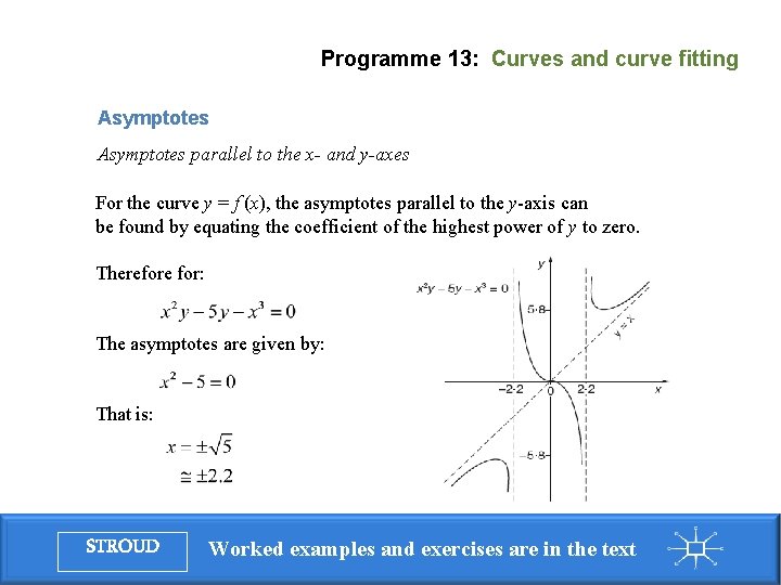
Programme 13: Curves and curve fitting Asymptotes parallel to the x- and y-axes For the curve y = f (x), the asymptotes parallel to the y-axis can be found by equating the coefficient of the highest power of y to zero. Therefore for: The asymptotes are given by: That is: STROUD Worked examples and exercises are in the text

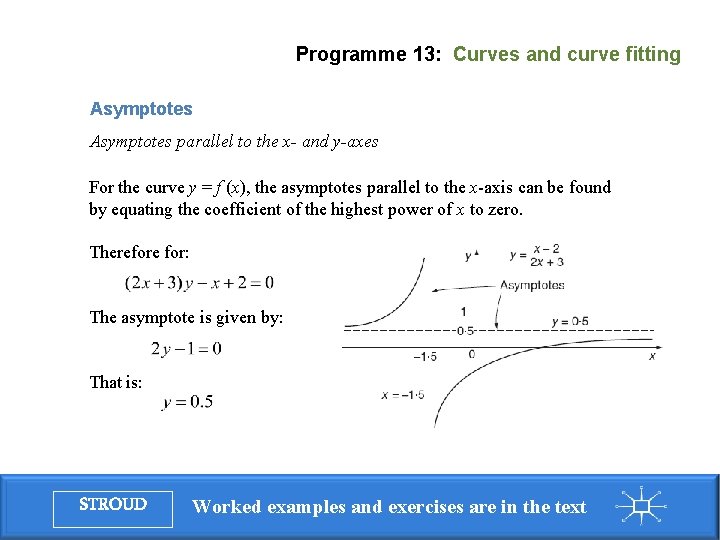
Programme 13: Curves and curve fitting Asymptotes parallel to the x- and y-axes For the curve y = f (x), the asymptotes parallel to the x-axis can be found by equating the coefficient of the highest power of x to zero. Therefore for: The asymptote is given by: That is: STROUD Worked examples and exercises are in the text

Programme 13: Curves and curve fitting Introduction Standard curves Asymptotes Systematic curve sketching, given the equation of the curve Curve fitting Method of least squares Correlation STROUD Worked examples and exercises are in the text

Programme 13: Curves and curve fitting Introduction Standard curves Asymptotes Systematic curve sketching, given the equation of the curve Curve fitting Method of least squares Correlation STROUD Worked examples and exercises are in the text

Programme 13: Curves and curve fitting Systematic curve sketching, given the equation of the curve Symmetry Intersection with the axes Change of origin Asymptotes Large and small values of x and y Stationary points Limitations STROUD Worked examples and exercises are in the text

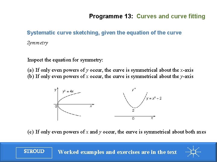
Programme 13: Curves and curve fitting Systematic curve sketching, given the equation of the curve Symmetry Inspect the equation for symmetry: (a) If only even powers of y occur, the curve is symmetrical about the x-axis (b) If only even powers of x occur, the curve is symmetrical about the y-axis (c) If only even powers of x and y occur, the curve is symmetrical about both axes STROUD Worked examples and exercises are in the text

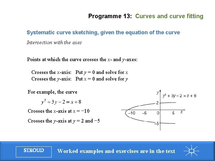
Programme 13: Curves and curve fitting Systematic curve sketching, given the equation of the curve Intersection with the axes Points at which the curve crosses the x- and y-axes: Crosses the x-axis: Put y = 0 and solve for x Crosses the y-axis: Put x = 0 and solve for y For example, the curve Crosses the x-axis at x = − 10 Crosses the y-axis at y = 2 and − 5 STROUD Worked examples and exercises are in the text

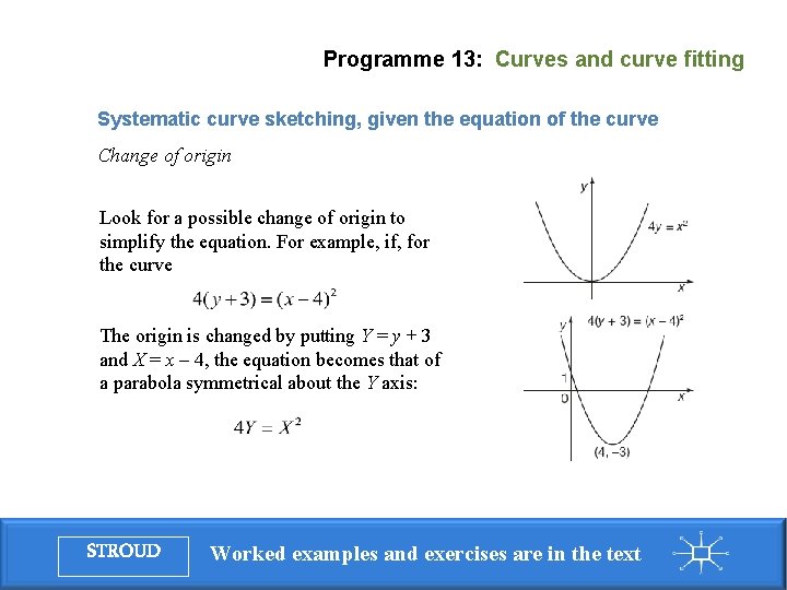
Programme 13: Curves and curve fitting Systematic curve sketching, given the equation of the curve Change of origin Look for a possible change of origin to simplify the equation. For example, if, for the curve The origin is changed by putting Y = y + 3 and X = x – 4, the equation becomes that of a parabola symmetrical about the Y axis: STROUD Worked examples and exercises are in the text

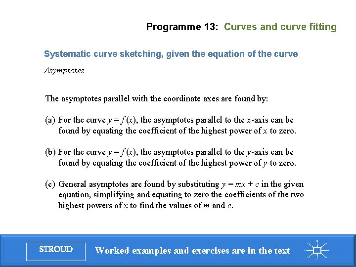
Programme 13: Curves and curve fitting Systematic curve sketching, given the equation of the curve Asymptotes The asymptotes parallel with the coordinate axes are found by: (a) For the curve y = f (x), the asymptotes parallel to the x-axis can be found by equating the coefficient of the highest power of x to zero. (b) For the curve y = f (x), the asymptotes parallel to the y-axis can be found by equating the coefficient of the highest power of y to zero. (c) General asymptotes are found by substituting y = mx + c in the given equation, simplifying and equating to zero the coefficients of the two highest powers of x to find the values of m and c. STROUD Worked examples and exercises are in the text

Programme 13: Curves and curve fitting Systematic curve sketching, given the equation of the curve Large and small values of x and y If x or y is small, higher powers of x or y become negligible and hence only lower powers of x or y appearing in the equation provide an approximate simpler form STROUD Worked examples and exercises are in the text

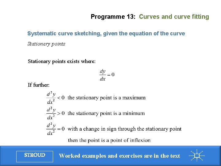
Programme 13: Curves and curve fitting Systematic curve sketching, given the equation of the curve Stationary points exists where: If further: STROUD Worked examples and exercises are in the text

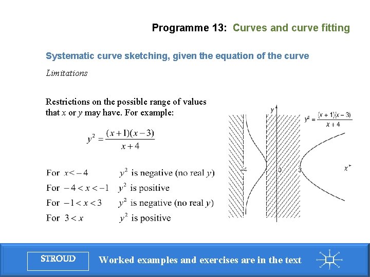
Programme 13: Curves and curve fitting Systematic curve sketching, given the equation of the curve Limitations Restrictions on the possible range of values that x or y may have. For example: STROUD Worked examples and exercises are in the text

Programme 13: Curves and curve fitting Introduction Standard curves Asymptotes Systematic curve sketching, given the equation of the curve Curve fitting Method of least squares Correlation STROUD Worked examples and exercises are in the text

Programme 13: Curves and curve fitting Introduction Standard curves Asymptotes Systematic curve sketching, given the equation of the curve Curve fitting Method of least squares Correlation STROUD Worked examples and exercises are in the text

Programme 13: Curves and curve fitting Curve fitting Readings of two related variables from a test or experiment normally include errors of various kinds and so the points that are plotted from the data are scattered about the positions they should ideally occupy. Having plotted the points a graph is then drawn through the scattered points to approximate to the relationship between the two variables. From the parameters involved in this graph an algebraic form for the relationship is then deduced. STROUD Worked examples and exercises are in the text

Programme 13: Curves and curve fitting Curve fitting Straight-line law Graphs of the form y = axn, where a and n are constants Graphs of the form y = aenx STROUD Worked examples and exercises are in the text

Programme 13: Curves and curve fitting Curve fitting Straight-line law If the assumption that the two variables x and y whose values are taken from experiment are linearly related then their relationship will be expressed algebraically as: where a represents the gradient of the straight line and b represents the vertical intercept From a plot of the data, a straight line is drawn through the data as the ‘line of best fit’. The values of a and b are then read off from the graph. STROUD Worked examples and exercises are in the text

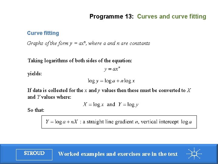
Programme 13: Curves and curve fitting Curve fitting Graphs of the form y = axn, where a and n are constants Taking logarithms of both sides of the equation: yields: If data is collected for the x and y values then these must be converted to X and Y values where: So that: STROUD Worked examples and exercises are in the text

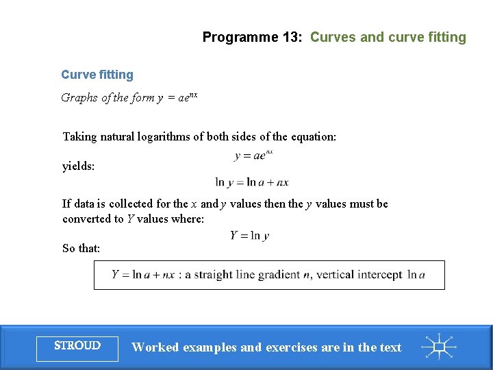
Programme 13: Curves and curve fitting Curve fitting Graphs of the form y = aenx Taking natural logarithms of both sides of the equation: yields: If data is collected for the x and y values then the y values must be converted to Y values where: So that: STROUD Worked examples and exercises are in the text

Programme 13: Curves and curve fitting Introduction Standard curves Asymptotes Systematic curve sketching, given the equation of the curve Curve fitting Method of least squares Correlation STROUD Worked examples and exercises are in the text

Programme 13: Curves and curve fitting Introduction Standard curves Asymptotes Systematic curve sketching, given the equation of the curve Curve fitting Method of least squares Correlation STROUD Worked examples and exercises are in the text

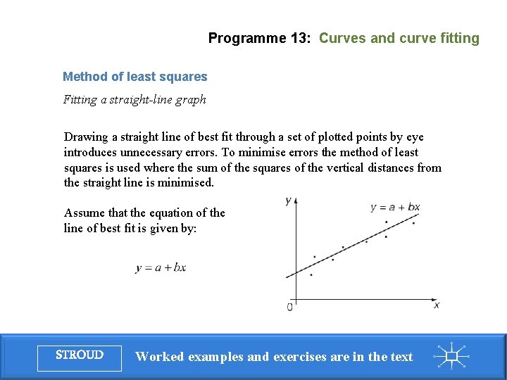
Programme 13: Curves and curve fitting Method of least squares Fitting a straight-line graph Drawing a straight line of best fit through a set of plotted points by eye introduces unnecessary errors. To minimise errors the method of least squares is used where the sum of the squares of the vertical distances from the straight line is minimised. Assume that the equation of the line of best fit is given by: STROUD Worked examples and exercises are in the text

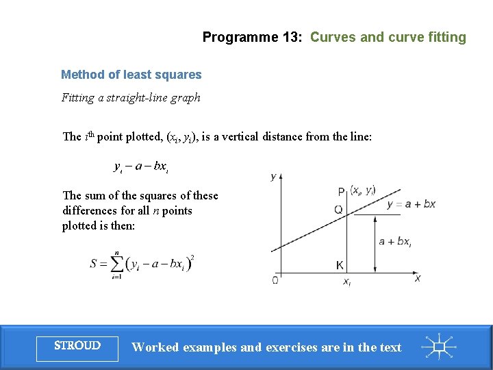
Programme 13: Curves and curve fitting Method of least squares Fitting a straight-line graph The ith point plotted, (xi, yi), is a vertical distance from the line: The sum of the squares of these differences for all n points plotted is then: STROUD Worked examples and exercises are in the text

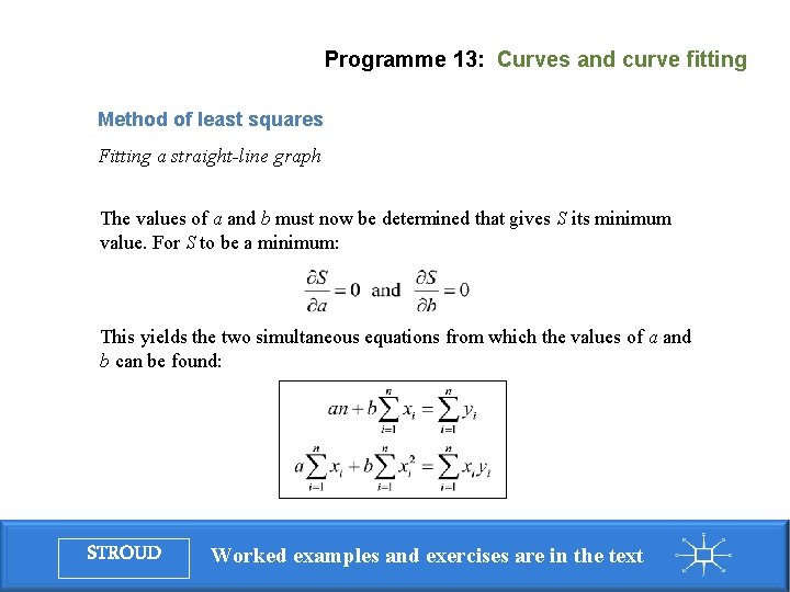
Programme 13: Curves and curve fitting Method of least squares Fitting a straight-line graph The values of a and b must now be determined that gives S its minimum value. For S to be a minimum: This yields the two simultaneous equations from which the values of a and b can be found: STROUD Worked examples and exercises are in the text

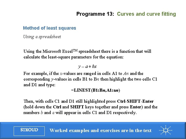
Programme 13: Curves and curve fitting Method of least squares Using a spreadsheet Using the Microsoft Excel. TM spreadsheet there is a function that will calculate the least-square parameters for the equation: For example, if the x-values are ranged in cells A 1 to An and the corresponding y-values in cells B 1 to Bn then highlight the two cells C 1 and D 1 and type: =LINEST(B 1: Bn, A 1: an) Then, with cells C 1 and D 1 still highlighted press Ctrl-SHIFT-Enter (hold down the Ctrl and SHIFT keys together and press Enter) and the numbers b and a will appear in cells C 1 and D 1 respectively. STROUD Worked examples and exercises are in the text

Programme 13: Curves and curve fitting Introduction Standard curves Asymptotes Systematic curve sketching, given the equation of the curve Curve fitting Method of least squares Correlation STROUD Worked examples and exercises are in the text

Programme 13: Curves and curve fitting Introduction Standard curves Asymptotes Systematic curve sketching, given the equation of the curve Curve fitting Method of least squares Correlation STROUD Worked examples and exercises are in the text

Programme 13: Curves and curve fitting Correlation If two variables vary together they are said to be correlated. For example, the fuel consumed by a car is correlated to the number of miles travelled. The exact relationship is not easily found because so many other factors are involved such as speed of travel, condition of the engine, tyre pressures and so on. What is important is that as the mileage increases so does the fuel used – there is a correlation. It is, however, most important to note that whilst cause-and-effect does display correlation between the cause and the effect as in the case of mileage travelled (cause) and petrol consumed (effect) the converse does not; the correlation of variables x and y does not imply cause-andeffect between x and y. STROUD Worked examples and exercises are in the text

Programme 13: Curves and curve fitting Correlation Measures of correlation The Pearson product-moment correlation coefficient Spearman’s rank correlation coefficient STROUD Worked examples and exercises are in the text

Programme 13: Curves and curve fitting Correlation Measures of correlation The strength of the correlation between two variables is given by a correlation coefficient – a number whose value ranges from − 1 to +1. The strongest positive correlation is when the correlation coefficient is +1 – in this case the two variables increase and decrease together in perfect unison. The strongest negative correlation is when the correlation coefficient is − 1 – in this case one variable will increase or decrease as the other decreases or increases respectively, again in perfect unison. When the correlation coefficient is zero then there is no correlation between the two variables whatsoever. STROUD Worked examples and exercises are in the text

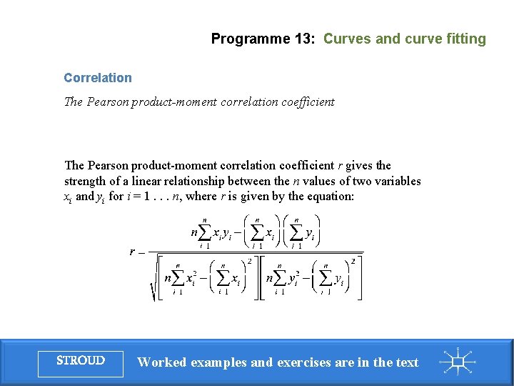
Programme 13: Curves and curve fitting Correlation The Pearson product-moment correlation coefficient r gives the strength of a linear relationship between the n values of two variables xi and yi for i = 1. . . n, where r is given by the equation: STROUD Worked examples and exercises are in the text

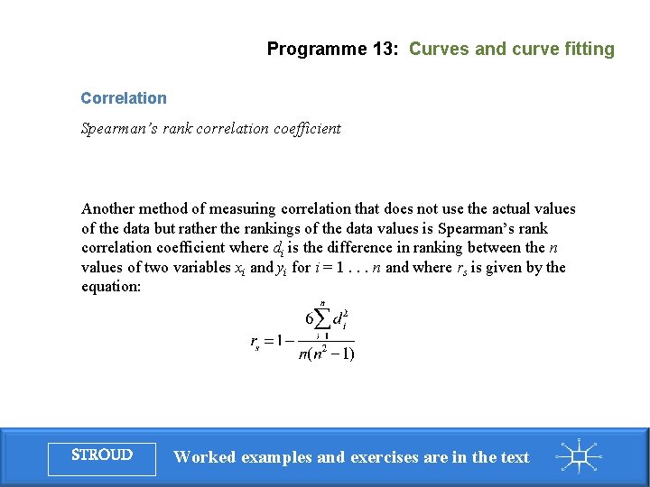
Programme 13: Curves and curve fitting Correlation Spearman’s rank correlation coefficient Another method of measuring correlation that does not use the actual values of the data but rather the rankings of the data values is Spearman’s rank correlation coefficient where di is the difference in ranking between the n values of two variables xi and yi for i = 1. . . n and where rs is given by the equation: STROUD Worked examples and exercises are in the text

Programme 13: Curves and curve fitting Learning outcomes üDraw sketch graphs of standard curves üDetermine the equations of asymptotes parallel to the x- and y-axes üSketch the graphs of curves with asymptotes, stationary points and other features üFit graphs to data using straight-line forms üFit graphs to data using the method of least squares üCalculate measures of correlation STROUD Worked examples and exercises are in the text