Curve with Curve Fitting with Polynomial Models How

Curve with Curve. Fitting with Polynomial Models • How do we use finite differences to determine the degree of a polynomial that will fit a given set of data? • How do we use technology to find polynomial models for a given set of data? Holt Mc. Dougal Algebra 2 Algebra 22 Holt Mc. Dougal

Curve Fitting with Polynomial Models Using Finite Differences to Determine Degree Use finite differences to determine the degree of the polynomial that best describes the data. The x-values increase by a constant 2. Find the differences of the y-values. 1. x y 8 10 7. 2 12 14 16 18 – 8. 3 – 19. 1 – 29 – 35. 8 First differences: – 6 – 9. 5 – 10. 8 – 9. 9 – 6. 8 Not constant Second differences: – 3. 5 – 1. 3 0. 9 3. 1 Not constant Third differences: 2. 2 Constant The third differences are constant. A cubic polynomial best describes the data. Holt Mc. Dougal Algebra 2

Curve Fitting with Polynomial Models Often, real-world data can be too irregular for you to use finite differences or find a polynomial function that fits perfectly. In these situations, you can use the regression feature of your graphing calculator. Remember that the closer the R 2 -value is to 1, the better the function fits the data. Holt Mc. Dougal Algebra 2

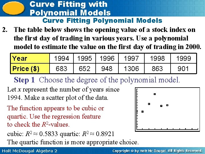
Curve Fitting with Polynomial Models Curve Fitting Polynomial Models 2. The table below shows the opening value of a stock index on the first day of trading in various years. Use a polynomial model to estimate the value on the first day of trading in 2000. Year Price ($) 1994 683 1995 652 1996 948 1997 1306 1998 863 1999 901 Step 1 Choose the degree of the polynomial model. Let x represent the number of years since 1994. Make a scatter plot of the data. The function appears to be cubic or quartic. Use the regression feature to check the R 2 -values. cubic: R 2 ≈ 0. 5833 quartic: R 2 ≈ 0. 8921 The quartic function is more appropriate choice. Holt Mc. Dougal Algebra 2

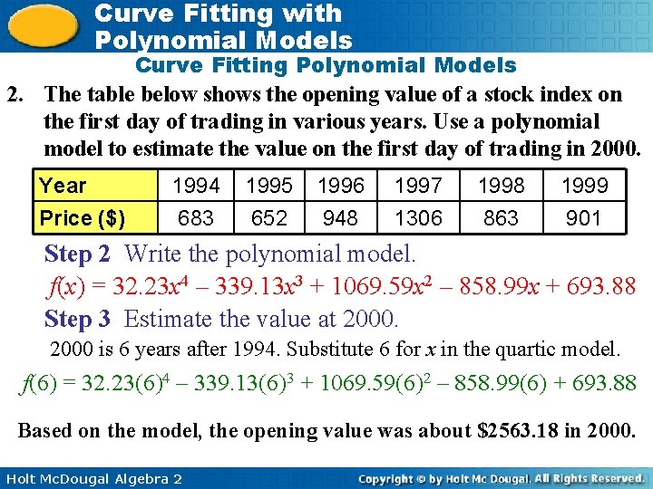
Curve Fitting with Polynomial Models Curve Fitting Polynomial Models 2. The table below shows the opening value of a stock index on the first day of trading in various years. Use a polynomial model to estimate the value on the first day of trading in 2000. Year Price ($) 1994 683 1995 652 1996 948 1997 1306 1998 863 1999 901 Step 2 Write the polynomial model. f(x) = 32. 23 x 4 – 339. 13 x 3 + 1069. 59 x 2 – 858. 99 x + 693. 88 Step 3 Estimate the value at 2000 is 6 years after 1994. Substitute 6 for x in the quartic model. f(6) = 32. 23(6)4 – 339. 13(6)3 + 1069. 59(6)2 – 858. 99(6) + 693. 88 Based on the model, the opening value was about $2563. 18 in 2000. Holt Mc. Dougal Algebra 2

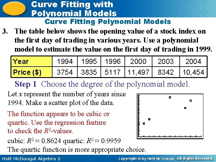
Curve Fitting with Polynomial Models Curve Fitting Polynomial Models 3. The table below shows the opening value of a stock index on the first day of trading in various years. Use a polynomial model to estimate the value on the first day of trading in 1999. Year Price ($) 1994 3754 1995 3835 1996 2000 5117 11, 497 2003 8342 2004 10, 454 Step 1 Choose the degree of the polynomial model. Let x represent the number of years since 1994. Make a scatter plot of the data. The function appears to be cubic or quartic. Use the regression feature to check the R 2 -values. cubic: R 2 ≈ 0. 8624 quartic: R 2 ≈ 0. 9959 The quartic function is more appropriate choice. Holt Mc. Dougal Algebra 2

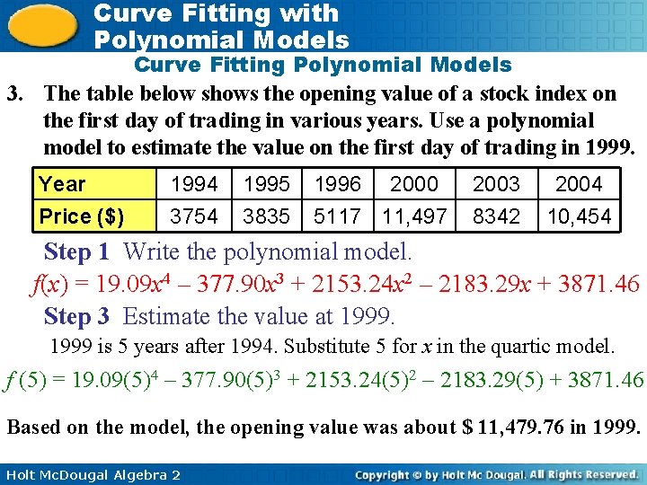
Curve Fitting with Polynomial Models Curve Fitting Polynomial Models 3. The table below shows the opening value of a stock index on the first day of trading in various years. Use a polynomial model to estimate the value on the first day of trading in 1999. Year Price ($) 1994 3754 1995 3835 1996 2000 5117 11, 497 2003 8342 2004 10, 454 Step 1 Write the polynomial model. f(x) = 19. 09 x 4 – 377. 90 x 3 + 2153. 24 x 2 – 2183. 29 x + 3871. 46 Step 3 Estimate the value at 1999 is 5 years after 1994. Substitute 5 for x in the quartic model. f (5) = 19. 09(5)4 – 377. 90(5)3 + 2153. 24(5)2 – 2183. 29(5) + 3871. 46 Based on the model, the opening value was about $ 11, 479. 76 in 1999. Holt Mc. Dougal Algebra 2

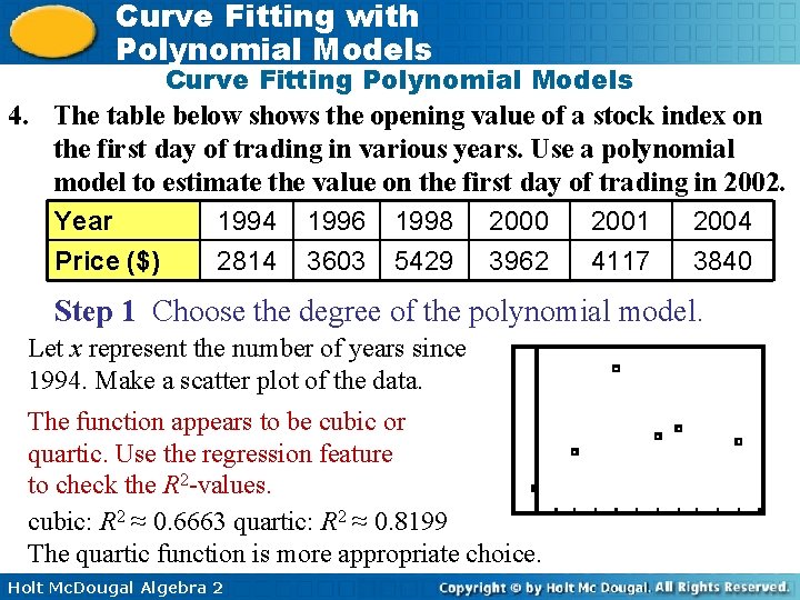
Curve Fitting with Polynomial Models Curve Fitting Polynomial Models 4. The table below shows the opening value of a stock index on the first day of trading in various years. Use a polynomial model to estimate the value on the first day of trading in 2002. Year 1994 1996 1998 2000 2001 2004 Price ($) 2814 3603 5429 3962 4117 3840 Step 1 Choose the degree of the polynomial model. Let x represent the number of years since 1994. Make a scatter plot of the data. The function appears to be cubic or quartic. Use the regression feature to check the R 2 -values. cubic: R 2 ≈ 0. 6663 quartic: R 2 ≈ 0. 8199 The quartic function is more appropriate choice. Holt Mc. Dougal Algebra 2

Curve Fitting with Polynomial Models Curve Fitting Polynomial Models 4. The table below shows the opening value of a stock index on the first day of trading in various years. Use a polynomial model to estimate the value on the first day of trading in 2002. Year 1994 1996 1998 2000 2001 2004 Price ($) 2814 3603 5429 3962 4117 3840 Step 1 Write the polynomial model. f(x) = 7. 08 x 4 – 126. 92 x 3 + 595. 95 x 2 – 241. 81 x + 2780. 54 Step 3 Estimate the value at 2002 is 8 years after 1994. Substitute 8 for x in the quartic model. f (8) = 7. 08(8)4 – 126. 92(8)3 + 595. 95(8)2 – 241. 81(8) + 2780. 54 Based on the model, the opening value was about $ 3003. 50 in 2002. Holt Mc. Dougal Algebra 2

Curve Fitting with Polynomial Models Lesson 15. 1 Practice B Holt Mc. Dougal Algebra 2