Computer Graphics Lecture 14 Curves and Surfaces II

Computer Graphics Lecture 14 Curves and Surfaces II

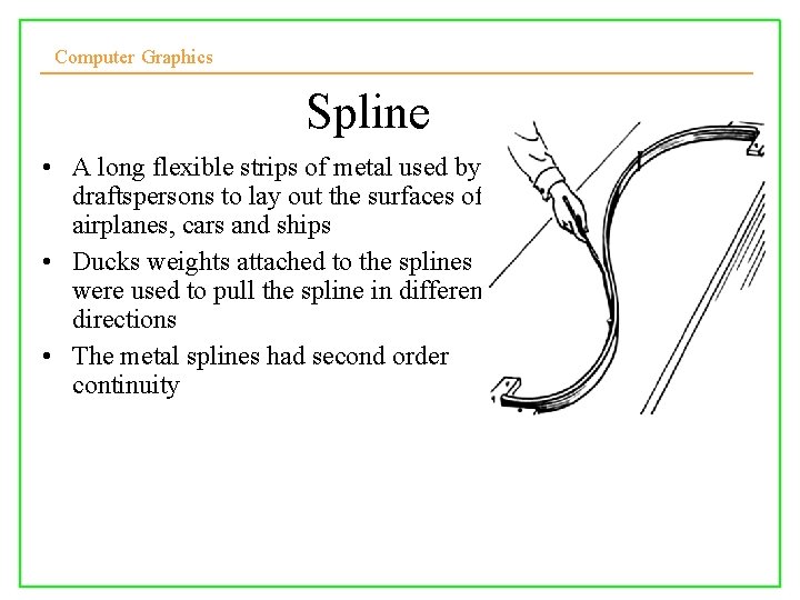
Computer Graphics Spline • A long flexible strips of metal used by draftspersons to lay out the surfaces of airplanes, cars and ships • Ducks weights attached to the splines were used to pull the spline in different directions • The metal splines had second order continuity 10/10/2008 Lecture 5 2

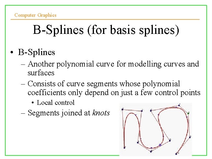
Computer Graphics B-Splines (for basis splines) • B-Splines – Another polynomial curve for modelling curves and surfaces – Consists of curve segments whose polynomial coefficients only depend on just a few control points • Local control – Segments joined at knots 10/10/2008 Lecture 5 3

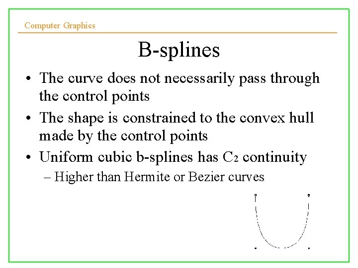
Computer Graphics B-splines • The curve does not necessarily pass through the control points • The shape is constrained to the convex hull made by the control points • Uniform cubic b-splines has C 2 continuity – Higher than Hermite or Bezier curves

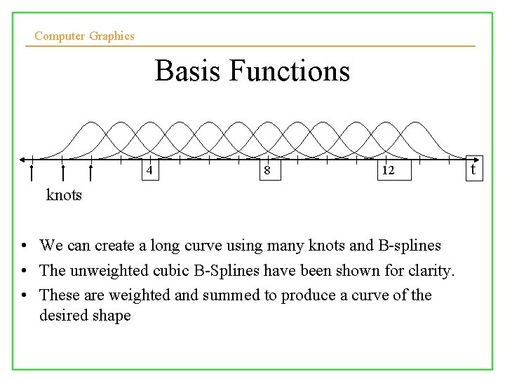
Computer Graphics Basis Functions 4 8 12 knots • We can create a long curve using many knots and B-splines • The unweighted cubic B-Splines have been shown for clarity. • These are weighted and summed to produce a curve of the desired shape 10/10/2008 Lecture 5 t

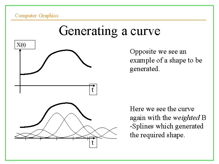
Computer Graphics Generating a curve X(t) Opposite we see an example of a shape to be generated. t Here we see the curve again with the weighted B -Splines which generated the required shape. t 10/10/2008 Lecture 5 6

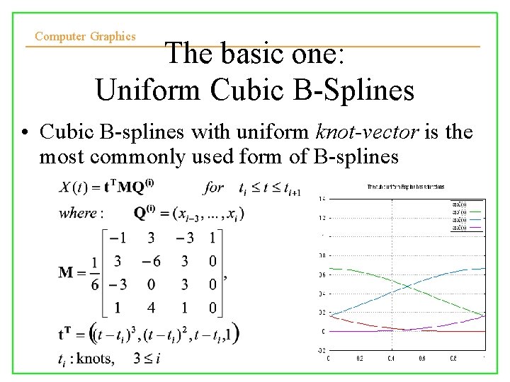
Computer Graphics The basic one: Uniform Cubic B-Splines • Cubic B-splines with uniform knot-vector is the most commonly used form of B-splines 10/10/2008 Lecture 5 7

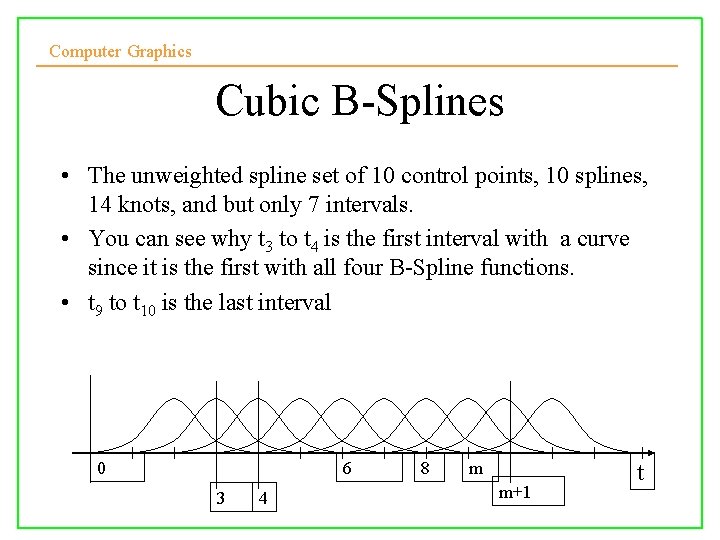
Computer Graphics Cubic B-Splines • The unweighted spline set of 10 control points, 10 splines, 14 knots, and but only 7 intervals. • You can see why t 3 to t 4 is the first interval with a curve since it is the first with all four B-Spline functions. • t 9 to t 10 is the last interval 0 10/10/2008 6 3 4 Lecture 5 8 m m+1 t 8

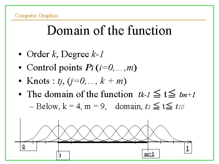
Computer Graphics Domain of the function • • Order k, Degree k-1 Control points Pi (i=0, …, m) Knots : tj, (j=0, …, k + m) The domain of the function tk-1 ≦ t≦ tm+1 – Below, k = 4, m = 9, domain, t 3 ≦ t≦ t 10 0 3 m+1 t

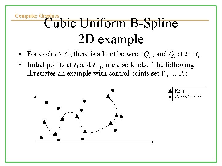
Computer Graphics Cubic Uniform B-Spline 2 D example • For each i 4 , there is a knot between Qi-1 and Qi at t = ti. • Initial points at t 3 and tm+1 are also knots. The following illustrates an example with control points set P 0 … P 9: Knot. Control point. 10/10/2008 Lecture 5 10

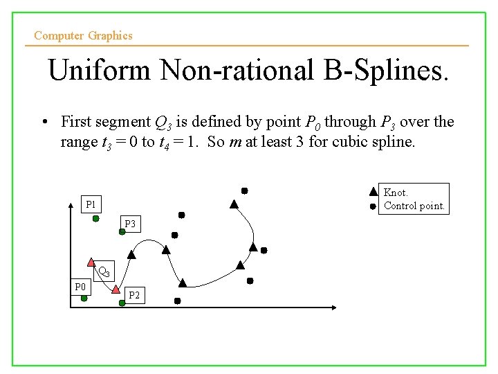
Computer Graphics Uniform Non-rational B-Splines. • First segment Q 3 is defined by point P 0 through P 3 over the range t 3 = 0 to t 4 = 1. So m at least 3 for cubic spline. Knot. Control point. P 1 P 3 Q 3 P 0 10/10/2008 P 2 Lecture 5 11

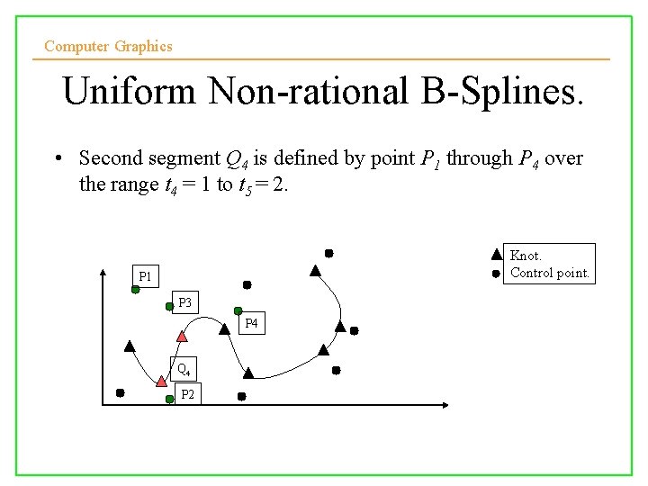
Computer Graphics Uniform Non-rational B-Splines. • Second segment Q 4 is defined by point P 1 through P 4 over the range t 4 = 1 to t 5 = 2. Knot. Control point. P 1 P 3 P 4 Q 4 P 2 10/10/2008 Lecture 5 12

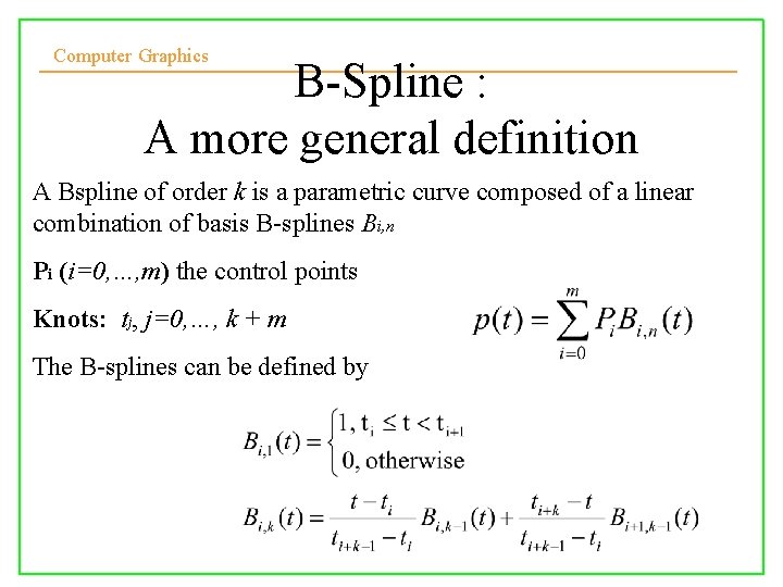
Computer Graphics B-Spline : A more general definition A Bspline of order k is a parametric curve composed of a linear combination of basis B-splines Bi, n Pi (i=0, …, m) the control points Knots: tj, j=0, …, k + m The B-splines can be defined by 10/10/2008 Lecture 5 13

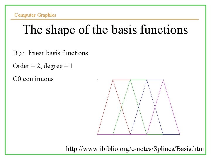
Computer Graphics The shape of the basis functions Bi, 2 : linear basis functions Order = 2, degree = 1 C 0 continuous 10/10/2008 Lecture 5 14 http: //www. ibiblio. org/e-notes/Splines/Basis. htm

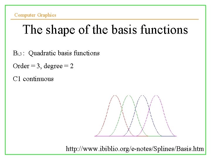
Computer Graphics The shape of the basis functions Bi, 3 : Quadratic basis functions Order = 3, degree = 2 C 1 continuous 10/10/2008 Lecture 5 15 http: //www. ibiblio. org/e-notes/Splines/Basis. htm

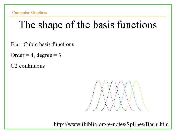
Computer Graphics The shape of the basis functions Bi, 4 : Cubic basis functions Order = 4, degree = 3 C 2 continuous 10/10/2008 Lecture 5 16 http: //www. ibiblio. org/e-notes/Splines/Basis. htm

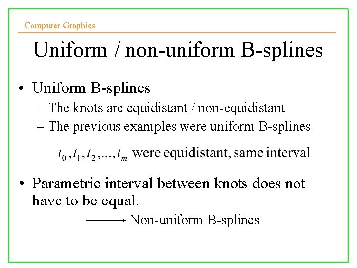
Computer Graphics Uniform / non-uniform B-splines • Uniform B-splines – The knots are equidistant / non-equidistant – The previous examples were uniform B-splines • Parametric interval between knots does not have to be equal. Non-uniform B-splines

Computer Graphics Non-uniform B-splines. • Blending functions no longer the same for each interval. • Advantages – Continuity at selected control points can be reduced to C 1 or lower – allows us to interpolate a control point without side-effects. – Can interpolate start and end points. – Easy to add extra knots and control points. • Good for shape modelling ! 10/10/2008

Computer Graphics Controlling the shape of the curves • Can control the shape through – Control points • Overlapping the control points to make it pass through a specific point – Knots • Changing the continuity by increasing the multiplicity at some knot (non-uniform bsplines)

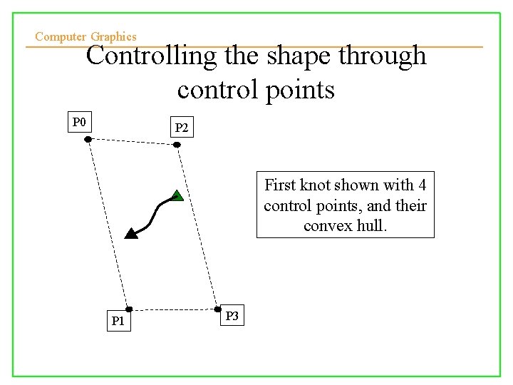
Computer Graphics Controlling the shape through control points P 0 P 2 First knot shown with 4 control points, and their convex hull. P 1 10/10/2008 P 3 Lecture 5 20

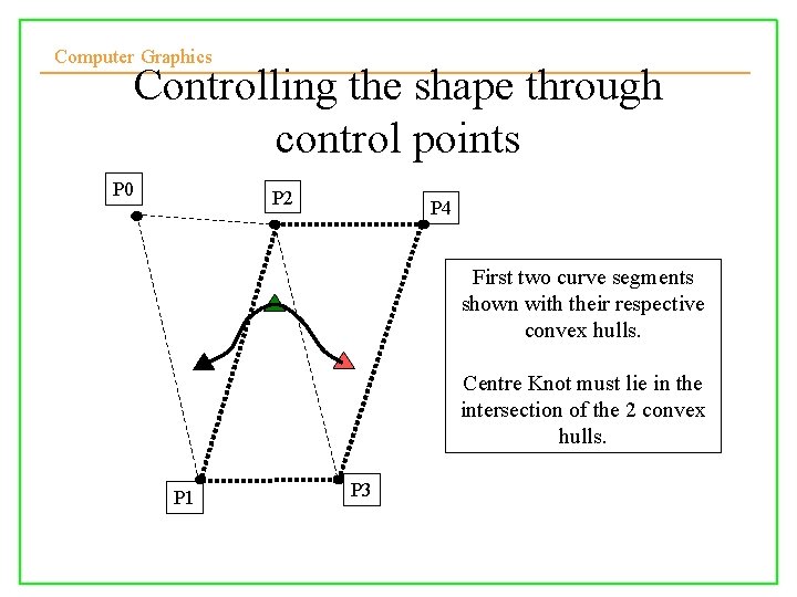
Computer Graphics Controlling the shape through control points P 0 P 2 P 4 First two curve segments shown with their respective convex hulls. Centre Knot must lie in the intersection of the 2 convex hulls. P 1 10/10/2008 P 3 Lecture 5 21

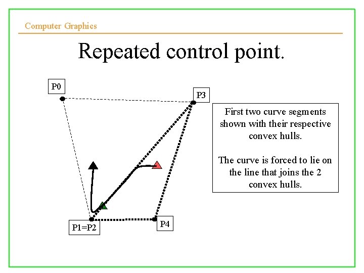
Computer Graphics Repeated control point. P 0 P 3 First two curve segments shown with their respective convex hulls. The curve is forced to lie on the line that joins the 2 convex hulls. P 1=P 2 10/10/2008 P 4 Lecture 5 22

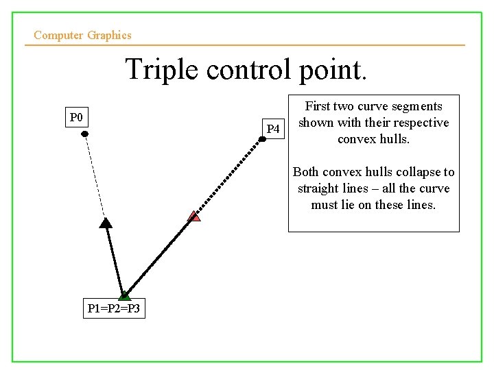
Computer Graphics Triple control point. P 0 P 4 First two curve segments shown with their respective convex hulls. Both convex hulls collapse to straight lines – all the curve must lie on these lines. P 1=P 2=P 3 10/10/2008 Lecture 5 23

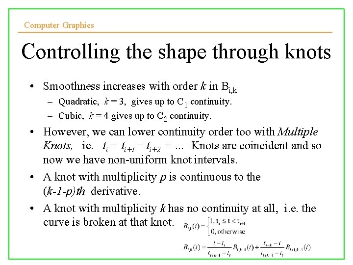
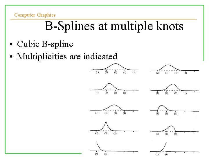
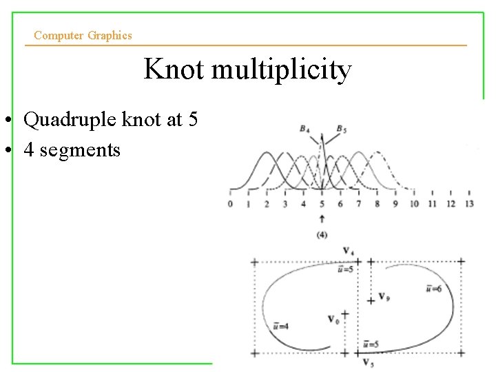
Computer Graphics Controlling the shape through knots • Smoothness increases with order k in Bi, k – Quadratic, k = 3, gives up to C 1 continuity. – Cubic, k = 4 gives up to C 2 continuity. • However, we can lower continuity order too with Multiple Knots, ie. ti = ti+1= ti+2 = … Knots are coincident and so now we have non-uniform knot intervals. • A knot with multiplicity p is continuous to the (k-1 -p)th derivative. • A knot with multiplicity k has no continuity at all, i. e. the curve is broken at that knot. 10/10/2008 Lecture 5 24

Computer Graphics B-Splines at multiple knots • Cubic B-spline • Multiplicities are indicated

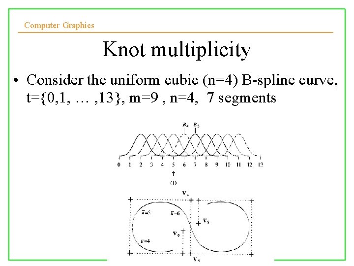
Computer Graphics Knot multiplicity • Consider the uniform cubic (n=4) B-spline curve, t={0, 1, … , 13}, m=9 , n=4, 7 segments

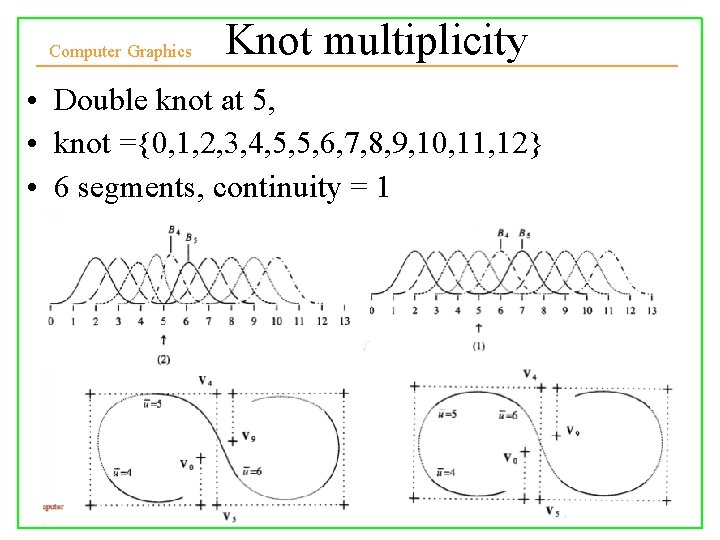
Computer Graphics Knot multiplicity • Double knot at 5, • knot ={0, 1, 2, 3, 4, 5, 5, 6, 7, 8, 9, 10, 11, 12} • 6 segments, continuity = 1

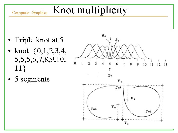
Computer Graphics Knot multiplicity • Triple knot at 5 • knot={0, 1, 2, 3, 4, 5, 5, 5, 6, 7, 8, 9, 10, 11} • 5 segments

Computer Graphics Knot multiplicity • Quadruple knot at 5 • 4 segments

Computer Graphics Summary of B-Splines. • Functions that can be manipulated by a series of control points with C 2 continuity and local control. • Don’t pass through their control points, although can be forced. • Uniform – Knots are equally spaced in t. • Non-Uniform – Knots are unequally spaced – Allows addition of extra control points anywhere in the set. 10/10/2008 Lecture 5 30

Computer Graphics Summary cont. • Do not have to worry about the continuity at the join points • For interactive curve modelling – B-Splines are very good. 10/10/2008 Lecture 5 31

Computer Graphics 2 nd Practical • Use Open. GL to draw the teapot • You must extend your code in the first assignment • Bonus marks for making it nice – Bump mapping – Texture mapping – Or whatever Deadline : 10 th December

Computer Graphics Reading for this lecture • Foley at al. , Chapter 11, sections 11. 2. 3, 11. 2. 4, 11. 2. 9, 11. 2. 10, 11. 3 and 11. 5. • Introductory text, Chapter 9, sections 9. 2. 4, 9. 2. 5, 9. 2. 7, 9. 2. 8 and 9. 3. . 10/10/2008 Lecture 5 33