Curve Fitting with Curving Fitting 6 9 Polynomial

Curve Fitting with Curving Fitting 6 -9 Polynomial Functions Warm Up Lesson Presentation Lesson Quiz Holt Algebra 22

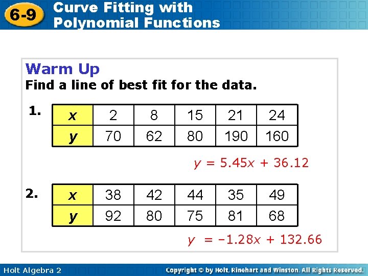
6 -9 Curve Fitting with Polynomial Functions Warm Up Find a line of best fit for the data. 1. x y 2 70 8 62 15 80 21 190 24 160 y = 5. 45 x + 36. 12 2. x y 38 92 42 80 44 75 35 81 49 68 y = – 1. 28 x + 132. 66 Holt Algebra 2

6 -9 Curve Fitting with Polynomial Functions Objectives Use finite differences to determine the degree of a polynomial that will fit a given set of data. Use technology to find polynomial models for a given set of data. Holt Algebra 2

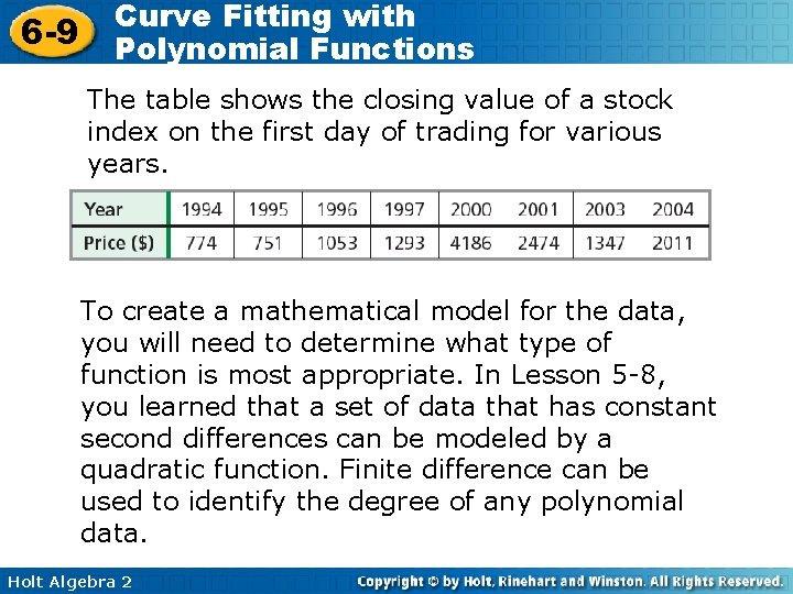
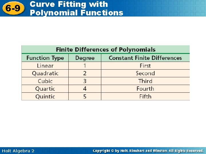
6 -9 Curve Fitting with Polynomial Functions The table shows the closing value of a stock index on the first day of trading for various years. To create a mathematical model for the data, you will need to determine what type of function is most appropriate. In Lesson 5 -8, you learned that a set of data that has constant second differences can be modeled by a quadratic function. Finite difference can be used to identify the degree of any polynomial data. Holt Algebra 2

6 -9 Curve Fitting with Polynomial Functions Holt Algebra 2

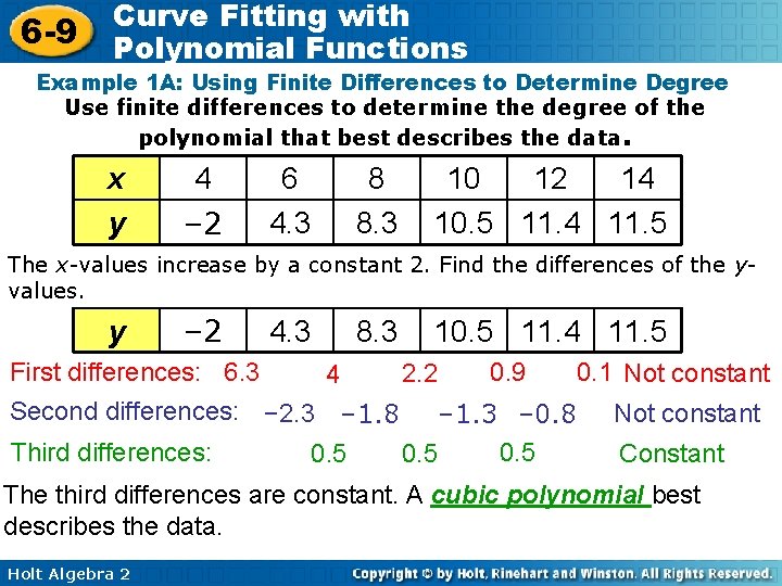
6 -9 Curve Fitting with Polynomial Functions Example 1 A: Using Finite Differences to Determine Degree Use finite differences to determine the degree of the polynomial that best describes the data. x y 4 – 2 6 4. 3 8 8. 3 10 12 14 10. 5 11. 4 11. 5 The x-values increase by a constant 2. Find the differences of the yvalues. y – 2 First differences: 6. 3 4. 3 8. 3 4 10. 5 11. 4 11. 5 2. 2 0. 9 0. 1 Not constant Second differences: – 2. 3 – 1. 8 – 1. 3 – 0. 8 Third differences: 0. 5 Not constant Constant The third differences are constant. A cubic polynomial best describes the data. Holt Algebra 2

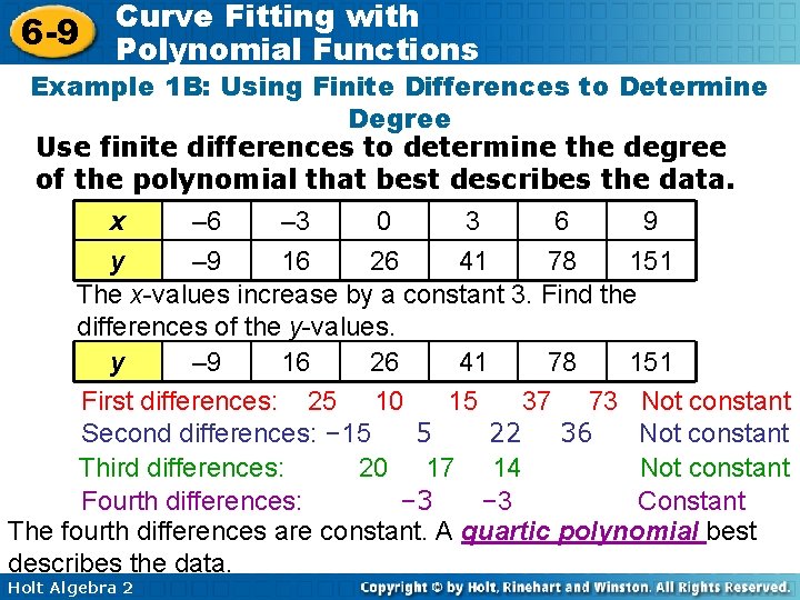
6 -9 Curve Fitting with Polynomial Functions Example 1 B: Using Finite Differences to Determine Degree Use finite differences to determine the degree of the polynomial that best describes the data. x – 6 – 3 0 3 6 9 y – 9 16 26 41 78 151 The x-values increase by a constant 3. Find the differences of the y-values. y – 9 16 26 41 78 151 First differences: 25 10 15 37 73 Not constant Second differences: – 15 5 22 36 Not constant Third differences: 20 17 14 Not constant Fourth differences: – 3 Constant The fourth differences are constant. A quartic polynomial best describes the data. Holt Algebra 2

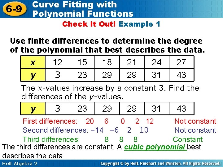
6 -9 Curve Fitting with Polynomial Functions Check It Out! Example 1 Use finite differences to determine the degree of the polynomial that best describes the data. x y 12 3 15 23 18 29 21 29 24 31 27 43 The x-values increase by a constant 3. Find the differences of the y-values. y 3 23 29 29 31 43 First differences: 20 6 0 2 12 Not constant Second differences: – 14 – 6 2 10 Not constant Third differences: 8 8 8 Constant The third differences are constant. A cubic polynomial best describes the data. Holt Algebra 2

6 -9 Curve Fitting with Polynomial Functions Once you have determined the degree of the polynomial that best describes the data, you can use your calculator to create the function. Holt Algebra 2

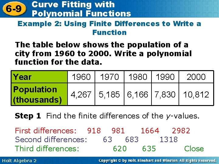
6 -9 Curve Fitting with Polynomial Functions Example 2: Using Finite Differences to Write a Function The table below shows the population of a city from 1960 to 2000. Write a polynomial function for the data. Year Population (thousands) 1960 1970 1980 1990 2000 4, 267 5, 185 6, 166 7, 830 10, 812 Step 1 Find the finite differences of the y-values. First differences: 918 981 1664 2982 Second differences: 63 683 1318 Third differences: 620 635 Close Holt Algebra 2

6 -9 Curve Fitting with Polynomial Functions Example 2 Continued Step 2 Determine the degree of the polynomial. Because third differences are relatively close, a cubic function should be a good model. Step 3 Use the cubic regression feature on your calculator. f(x) ≈ 104. 58 x 3 – 283. 86 x 2 + 1098. 34 x + 4266. 79 Holt Algebra 2

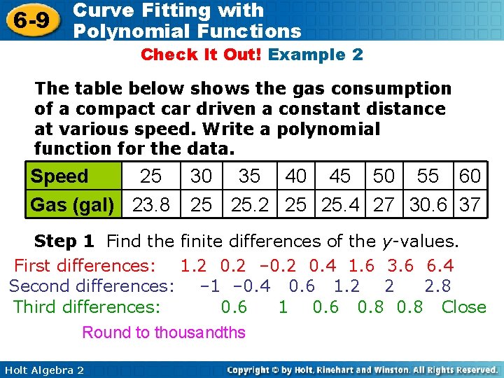
6 -9 Curve Fitting with Polynomial Functions Check It Out! Example 2 The table below shows the gas consumption of a compact car driven a constant distance at various speed. Write a polynomial function for the data. Speed 25 Gas (gal) 23. 8 30 35 40 45 50 55 60 25 25. 2 25 25. 4 27 30. 6 37 Step 1 Find the finite differences of the y-values. First differences: 1. 2 0. 2 – 0. 2 0. 4 1. 6 3. 6 6. 4 Second differences: – 1 – 0. 4 0. 6 1. 2 2 2. 8 Third differences: 0. 6 1 0. 6 0. 8 Close Round to thousandths Holt Algebra 2

6 -9 Curve Fitting with Polynomial Functions Check It Out! Example 2 Continued Step 2 Determine the degree of the polynomial. Because third differences are relatively close, a cubic function should be a good model. Step 3 Use the cubic regression feature on your calculator. f(x) ≈ 0. 001 x 3 – 0. 113 x 2 + 4. 134 x - 24. 867 Holt Algebra 2

6 -9 Curve Fitting with Polynomial Functions Often, real-world data can be too irregular for you to use finite differences or find a polynomial function that fits perfectly. In these situations, you can use the regression feature of your graphing calculator. Remember that the closer the R 2 -value is to 1, the better the function fits the data. Holt Algebra 2

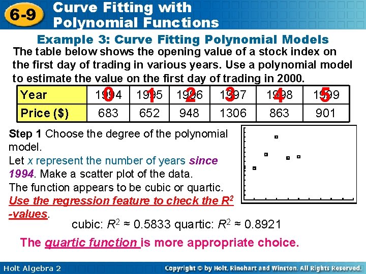
6 -9 Curve Fitting with Polynomial Functions Example 3: Curve Fitting Polynomial Models The table below shows the opening value of a stock index on the first day of trading in various years. Use a polynomial model to estimate the value on the first day of trading in 2000. Year Price ($) 0 1994 683 1 1995 652 2 1996 948 3 1997 1306 4 1998 863 Step 1 Choose the degree of the polynomial model. Let x represent the number of years since 1994. Make a scatter plot of the data. The function appears to be cubic or quartic. Use the regression feature to check the R 2 -values. cubic: R 2 ≈ 0. 5833 quartic: R 2 ≈ 0. 8921 The quartic function is more appropriate choice. Holt Algebra 2 5 1999 901

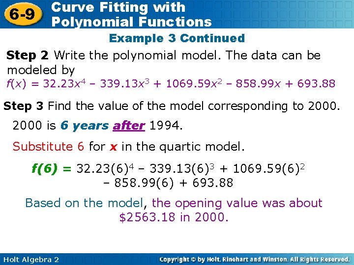
6 -9 Curve Fitting with Polynomial Functions Example 3 Continued Step 2 Write the polynomial model. The data can be modeled by f(x) = 32. 23 x 4 – 339. 13 x 3 + 1069. 59 x 2 – 858. 99 x + 693. 88 Step 3 Find the value of the model corresponding to 2000 is 6 years after 1994. Substitute 6 for x in the quartic model. f(6) = 32. 23(6)4 – 339. 13(6)3 + 1069. 59(6)2 – 858. 99(6) + 693. 88 Based on the model, the opening value was about $2563. 18 in 2000. Holt Algebra 2

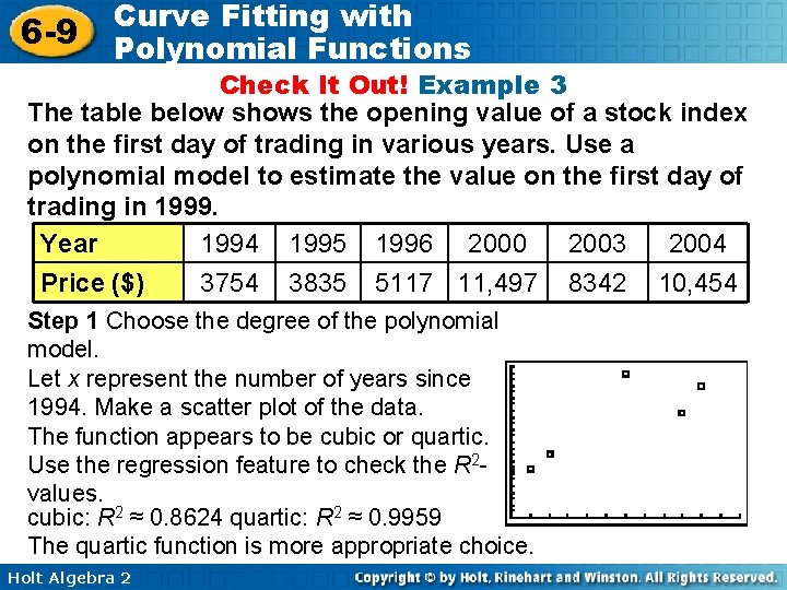
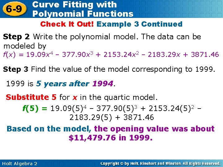
6 -9 Curve Fitting with Polynomial Functions Check It Out! Example 3 The table below shows the opening value of a stock index on the first day of trading in various years. Use a polynomial model to estimate the value on the first day of trading in 1999. Year 1994 1995 1996 2000 2003 2004 Price ($) 3754 3835 5117 11, 497 8342 10, 454 Step 1 Choose the degree of the polynomial model. Let x represent the number of years since 1994. Make a scatter plot of the data. The function appears to be cubic or quartic. Use the regression feature to check the R 2 values. cubic: R 2 ≈ 0. 8624 quartic: R 2 ≈ 0. 9959 The quartic function is more appropriate choice. Holt Algebra 2

6 -9 Curve Fitting with Polynomial Functions Check It Out! Example 3 Continued Step 2 Write the polynomial model. The data can be modeled by f(x) = 19. 09 x 4 – 377. 90 x 3 + 2153. 24 x 2 – 2183. 29 x + 3871. 46 Step 3 Find the value of the model corresponding to 1999 is 5 years after 1994. Substitute 5 for x in the quartic model. f(5) = 19. 09(5)4 – 377. 90(5)3 + 2153. 24(5)2 – 2183. 29(5) + 3871. 46 Based on the model, the opening value was about $11, 479. 76 in 1999. Holt Algebra 2

6 -9 Curve Fitting with Polynomial Functions Lesson Quiz: Part I 1. Use finite differences to determine the degree of the polynomial that best describes the data. x y cubic Holt Algebra 2 8 7. 2 10 12 14 16 18 1. 2 – 8. 3 – 19. 1 – 29 – 35. 8

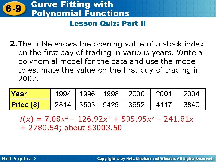
6 -9 Curve Fitting with Polynomial Functions Lesson Quiz: Part II 2. The table shows the opening value of a stock index on the first day of trading in various years. Write a polynomial model for the data and use the model to estimate the value on the first day of trading in 2002. Year Price ($) 1994 2814 1996 3603 1998 5429 2000 3962 2001 4117 2004 3840 f(x) = 7. 08 x 4 – 126. 92 x 3 + 595. 95 x 2 – 241. 81 x + 2780. 54; about $3003. 50 Holt Algebra 2