Railway Curves Transition Curves Transition Curves An easement
![Railway Curves Railway Curves](https://slidetodoc.com/presentation_image_h2/c1a8ddc073bce1675e4bd1ae2348660b/image-1.jpg)
![Transition Curves Transition Curves](https://slidetodoc.com/presentation_image_h2/c1a8ddc073bce1675e4bd1ae2348660b/image-2.jpg)
![Transition Curves An easement curve, introduced between straight & curved track to facilitate gradual Transition Curves An easement curve, introduced between straight & curved track to facilitate gradual](https://slidetodoc.com/presentation_image_h2/c1a8ddc073bce1675e4bd1ae2348660b/image-3.jpg)
![Key Design Parameters for Transition Curves Rate of Change of Actual Cant (RCa) mm/s, Key Design Parameters for Transition Curves Rate of Change of Actual Cant (RCa) mm/s,](https://slidetodoc.com/presentation_image_h2/c1a8ddc073bce1675e4bd1ae2348660b/image-4.jpg)
![Requirements from Transition Curves • Curvature shall vary uniformly with distance – Curvature = Requirements from Transition Curves • Curvature shall vary uniformly with distance – Curvature =](https://slidetodoc.com/presentation_image_h2/c1a8ddc073bce1675e4bd1ae2348660b/image-5.jpg)
![Transition Curves • The spiral (Clothoid), which changes the direction angle uniformly along length, Transition Curves • The spiral (Clothoid), which changes the direction angle uniformly along length,](https://slidetodoc.com/presentation_image_h2/c1a8ddc073bce1675e4bd1ae2348660b/image-6.jpg)
![Transition Curves • There is not much difference in the layout of a spiral Transition Curves • There is not much difference in the layout of a spiral](https://slidetodoc.com/presentation_image_h2/c1a8ddc073bce1675e4bd1ae2348660b/image-7.jpg)
![Desirable Versine and Cant Diagram Cubic Parabola – Curvature changes linearly v Ca Transition Desirable Versine and Cant Diagram Cubic Parabola – Curvature changes linearly v Ca Transition](https://slidetodoc.com/presentation_image_h2/c1a8ddc073bce1675e4bd1ae2348660b/image-8.jpg)
![Shift Transition Curves Inserting Transition Curves Shift Transition Curves Inserting Transition Curves](https://slidetodoc.com/presentation_image_h2/c1a8ddc073bce1675e4bd1ae2348660b/image-9.jpg)
![Shift Due to Transition Curve Circular Curve With Transition Extended Circular Curve C D Shift Due to Transition Curve Circular Curve With Transition Extended Circular Curve C D](https://slidetodoc.com/presentation_image_h2/c1a8ddc073bce1675e4bd1ae2348660b/image-10.jpg)
![Length of Transition Curve Length of Transition Curve](https://slidetodoc.com/presentation_image_h2/c1a8ddc073bce1675e4bd1ae2348660b/image-11.jpg)
![](https://slidetodoc.com/presentation_image_h2/c1a8ddc073bce1675e4bd1ae2348660b/image-12.jpg)
![Length of Transition Curve • Comfort Criteria: Rate of Change of Cd (RCd) – Length of Transition Curve • Comfort Criteria: Rate of Change of Cd (RCd) –](https://slidetodoc.com/presentation_image_h2/c1a8ddc073bce1675e4bd1ae2348660b/image-13.jpg)
![Length of Transition Curve • Comfort Criteria: Rate of Change of Cd (RCd) – Length of Transition Curve • Comfort Criteria: Rate of Change of Cd (RCd) –](https://slidetodoc.com/presentation_image_h2/c1a8ddc073bce1675e4bd1ae2348660b/image-14.jpg)
![Length of Transition Curve • Comfort Criteria: Rate of Change of Ca (RCa) – Length of Transition Curve • Comfort Criteria: Rate of Change of Ca (RCa) –](https://slidetodoc.com/presentation_image_h2/c1a8ddc073bce1675e4bd1ae2348660b/image-15.jpg)
![Length of Transition Curve • Safety Criteria (Twist) – Cant gradient causes twist in Length of Transition Curve • Safety Criteria (Twist) – Cant gradient causes twist in](https://slidetodoc.com/presentation_image_h2/c1a8ddc073bce1675e4bd1ae2348660b/image-16.jpg)
![Length of Transition Curve • Length of transition will be maximum of L 1 Length of Transition Curve • Length of transition will be maximum of L 1](https://slidetodoc.com/presentation_image_h2/c1a8ddc073bce1675e4bd1ae2348660b/image-17.jpg)
![Length of Transition Curve • Length of transition will be maximum of L 1 Length of Transition Curve • Length of transition will be maximum of L 1](https://slidetodoc.com/presentation_image_h2/c1a8ddc073bce1675e4bd1ae2348660b/image-18.jpg)
![Length of Transition Curve • In exceptional circumstances, minimum length of transition will be Length of Transition Curve • In exceptional circumstances, minimum length of transition will be](https://slidetodoc.com/presentation_image_h2/c1a8ddc073bce1675e4bd1ae2348660b/image-19.jpg)
![Procedure to find Speed on Curve • Find equilibrium cant for the maximum speed Procedure to find Speed on Curve • Find equilibrium cant for the maximum speed](https://slidetodoc.com/presentation_image_h2/c1a8ddc073bce1675e4bd1ae2348660b/image-20.jpg)
![Procedure to find Speed on Curve • Cant to be Provided shall also be Procedure to find Speed on Curve • Cant to be Provided shall also be](https://slidetodoc.com/presentation_image_h2/c1a8ddc073bce1675e4bd1ae2348660b/image-21.jpg)
![Exercise Find Maximum Permissible Speed for – BG route having Speed Potential = 130 Exercise Find Maximum Permissible Speed for – BG route having Speed Potential = 130](https://slidetodoc.com/presentation_image_h2/c1a8ddc073bce1675e4bd1ae2348660b/image-22.jpg)
![Exercise Find Desirable and Minimum Transition Length for – BG route having Speed Potential Exercise Find Desirable and Minimum Transition Length for – BG route having Speed Potential](https://slidetodoc.com/presentation_image_h2/c1a8ddc073bce1675e4bd1ae2348660b/image-23.jpg)
![Exercise Calculate Shift for – BG route having Speed Potential = 130 Kmph Rajdhani Exercise Calculate Shift for – BG route having Speed Potential = 130 Kmph Rajdhani](https://slidetodoc.com/presentation_image_h2/c1a8ddc073bce1675e4bd1ae2348660b/image-24.jpg)
![Desirable Versine and Cant Diagram V Transition Ca Transition Desirable Versine and Cant Diagram V Transition Ca Transition](https://slidetodoc.com/presentation_image_h2/c1a8ddc073bce1675e4bd1ae2348660b/image-25.jpg)
![If there is no Transition Curve ? v Transition Ca Transition How to introduce If there is no Transition Curve ? v Transition Ca Transition How to introduce](https://slidetodoc.com/presentation_image_h2/c1a8ddc073bce1675e4bd1ae2348660b/image-26.jpg)
![~2 m ? V Virtual Transition ~2 m ? V Virtual Transition](https://slidetodoc.com/presentation_image_h2/c1a8ddc073bce1675e4bd1ae2348660b/image-27.jpg)
![Virtual Transition • If there is no space for transition, circular curve immediately follows Virtual Transition • If there is no space for transition, circular curve immediately follows](https://slidetodoc.com/presentation_image_h2/c1a8ddc073bce1675e4bd1ae2348660b/image-28.jpg)
![Reverse and Compound Curves Reverse and Compound Curves](https://slidetodoc.com/presentation_image_h2/c1a8ddc073bce1675e4bd1ae2348660b/image-29.jpg)
![Reverse Curves Length of intermediate Transition will be Maximum of L 1 = 0. Reverse Curves Length of intermediate Transition will be Maximum of L 1 = 0.](https://slidetodoc.com/presentation_image_h2/c1a8ddc073bce1675e4bd1ae2348660b/image-30.jpg)
![Reverse Curves • For high speeds in Group A and B routes a straight Reverse Curves • For high speeds in Group A and B routes a straight](https://slidetodoc.com/presentation_image_h2/c1a8ddc073bce1675e4bd1ae2348660b/image-31.jpg)
![Compound Curves Compound Curves](https://slidetodoc.com/presentation_image_h2/c1a8ddc073bce1675e4bd1ae2348660b/image-32.jpg)
![Compound and Reverse Curves • For Compound Curves: Length of Intermediate Transition shall be Compound and Reverse Curves • For Compound Curves: Length of Intermediate Transition shall be](https://slidetodoc.com/presentation_image_h2/c1a8ddc073bce1675e4bd1ae2348660b/image-33.jpg)
![Vertical curves Vertical curves](https://slidetodoc.com/presentation_image_h2/c1a8ddc073bce1675e4bd1ae2348660b/image-34.jpg)
![Types of Vertical Curves Types of Vertical Curves](https://slidetodoc.com/presentation_image_h2/c1a8ddc073bce1675e4bd1ae2348660b/image-35.jpg)
![Vertical curves • Vertical Curves to be provided, if ; Algebraic Difference between the Vertical curves • Vertical Curves to be provided, if ; Algebraic Difference between the](https://slidetodoc.com/presentation_image_h2/c1a8ddc073bce1675e4bd1ae2348660b/image-36.jpg)
![Vertical curves • Important issues – Vertical acceleration – Drainage (Sag) – Ventilation (Summit) Vertical curves • Important issues – Vertical acceleration – Drainage (Sag) – Ventilation (Summit)](https://slidetodoc.com/presentation_image_h2/c1a8ddc073bce1675e4bd1ae2348660b/image-37.jpg)
![Vertical curves • Shall be as flat as possible to reduce Discomfort to passengers Vertical curves • Shall be as flat as possible to reduce Discomfort to passengers](https://slidetodoc.com/presentation_image_h2/c1a8ddc073bce1675e4bd1ae2348660b/image-38.jpg)
![Effects of curve: Curve Resistance Effects of curve: Curve Resistance](https://slidetodoc.com/presentation_image_h2/c1a8ddc073bce1675e4bd1ae2348660b/image-39.jpg)
![Compensation for Curvature on gradient • Known as Grade Compensation – Reduction in ruling Compensation for Curvature on gradient • Known as Grade Compensation – Reduction in ruling](https://slidetodoc.com/presentation_image_h2/c1a8ddc073bce1675e4bd1ae2348660b/image-40.jpg)
![Check Rails on Curves Check Rails on Curves](https://slidetodoc.com/presentation_image_h2/c1a8ddc073bce1675e4bd1ae2348660b/image-41.jpg)
![Check Rails on Curves CLEARANCE Too Much Wear on Outer Rail in Sharp Curves; Check Rails on Curves CLEARANCE Too Much Wear on Outer Rail in Sharp Curves;](https://slidetodoc.com/presentation_image_h2/c1a8ddc073bce1675e4bd1ae2348660b/image-42.jpg)
![Thank You Thank You](https://slidetodoc.com/presentation_image_h2/c1a8ddc073bce1675e4bd1ae2348660b/image-43.jpg)
![IRPWM Provisions • Inspections – AEN to inspect one curve in each PWI jurisdiction IRPWM Provisions • Inspections – AEN to inspect one curve in each PWI jurisdiction](https://slidetodoc.com/presentation_image_h2/c1a8ddc073bce1675e4bd1ae2348660b/image-44.jpg)
![IRPWM Provisions (BG) • Lateral wear on Rails in Curves (301(b)(iv)) – Group A IRPWM Provisions (BG) • Lateral wear on Rails in Curves (301(b)(iv)) – Group A](https://slidetodoc.com/presentation_image_h2/c1a8ddc073bce1675e4bd1ae2348660b/image-45.jpg)
![IRPWM Provisions (BG) • Cut in rails in SWR track (424) – To make IRPWM Provisions (BG) • Cut in rails in SWR track (424) – To make](https://slidetodoc.com/presentation_image_h2/c1a8ddc073bce1675e4bd1ae2348660b/image-46.jpg)
![IRPWM Provisions (BG) After relaying • On curves, Versine variation over Theoretical versine on IRPWM Provisions (BG) After relaying • On curves, Versine variation over Theoretical versine on](https://slidetodoc.com/presentation_image_h2/c1a8ddc073bce1675e4bd1ae2348660b/image-47.jpg)
![IRPWM Provisions (BG) In-service • Gauge (224(2)(e)(v)) – On straight : (-) 6 mm IRPWM Provisions (BG) In-service • Gauge (224(2)(e)(v)) – On straight : (-) 6 mm](https://slidetodoc.com/presentation_image_h2/c1a8ddc073bce1675e4bd1ae2348660b/image-48.jpg)
![IRPWM Provisions (BG) In-service tolerances (speed >100 kmph, <140 kmph) • Twist (607(2)(iii)) – IRPWM Provisions (BG) In-service tolerances (speed >100 kmph, <140 kmph) • Twist (607(2)(iii)) –](https://slidetodoc.com/presentation_image_h2/c1a8ddc073bce1675e4bd1ae2348660b/image-49.jpg)
![IRPWM Provisions (BG) In-service tolerances (speed >100 kmph, <140 kmph) • Alignment defect (607(2)(i)) IRPWM Provisions (BG) In-service tolerances (speed >100 kmph, <140 kmph) • Alignment defect (607(2)(i))](https://slidetodoc.com/presentation_image_h2/c1a8ddc073bce1675e4bd1ae2348660b/image-50.jpg)
![IRPWM Provisions • Radius of curve (401(1)) R = 125*C 2/V • For measuring IRPWM Provisions • Radius of curve (401(1)) R = 125*C 2/V • For measuring](https://slidetodoc.com/presentation_image_h2/c1a8ddc073bce1675e4bd1ae2348660b/image-51.jpg)
![IRPWM Provisions • Safe speed on a Curve (405(1)(a)) V = 0. 27 √{R IRPWM Provisions • Safe speed on a Curve (405(1)(a)) V = 0. 27 √{R](https://slidetodoc.com/presentation_image_h2/c1a8ddc073bce1675e4bd1ae2348660b/image-52.jpg)
![IRPWM Provisions • Curve boards(409(1)) – Curve board shall be provided at tangent point IRPWM Provisions • Curve boards(409(1)) – Curve board shall be provided at tangent point](https://slidetodoc.com/presentation_image_h2/c1a8ddc073bce1675e4bd1ae2348660b/image-53.jpg)
![Curve Board Curve Board](https://slidetodoc.com/presentation_image_h2/c1a8ddc073bce1675e4bd1ae2348660b/image-54.jpg)
![IRPWM Provisions • Super-elevation marking on rails (409(3)) – Value of super-elevation shall be IRPWM Provisions • Super-elevation marking on rails (409(3)) – Value of super-elevation shall be](https://slidetodoc.com/presentation_image_h2/c1a8ddc073bce1675e4bd1ae2348660b/image-55.jpg)
![Lead Curve following Turnout • Minimum radius of lead curve (410(2)) : 350 m Lead Curve following Turnout • Minimum radius of lead curve (410(2)) : 350 m](https://slidetodoc.com/presentation_image_h2/c1a8ddc073bce1675e4bd1ae2348660b/image-56.jpg)
![Lead portion and Turn-in curves The variation in versine on two successive stations in Lead portion and Turn-in curves The variation in versine on two successive stations in](https://slidetodoc.com/presentation_image_h2/c1a8ddc073bce1675e4bd1ae2348660b/image-57.jpg)
![Thank You Thank You](https://slidetodoc.com/presentation_image_h2/c1a8ddc073bce1675e4bd1ae2348660b/image-58.jpg)
![Extra Clearances on curves Lean and Sway Extra Clearances on curves Lean and Sway](https://slidetodoc.com/presentation_image_h2/c1a8ddc073bce1675e4bd1ae2348660b/image-59.jpg)
![Clearances on curves : Lean L = H * Ca/G H = height of Clearances on curves : Lean L = H * Ca/G H = height of](https://slidetodoc.com/presentation_image_h2/c1a8ddc073bce1675e4bd1ae2348660b/image-60.jpg)
![Clearances on curves : Additional Allowance due to Lurch & Sway • Inside of Clearances on curves : Additional Allowance due to Lurch & Sway • Inside of](https://slidetodoc.com/presentation_image_h2/c1a8ddc073bce1675e4bd1ae2348660b/image-61.jpg)
![Extra Clearances on Curves: Platforms and structures Extra Clearances on Curves: Platforms and structures](https://slidetodoc.com/presentation_image_h2/c1a8ddc073bce1675e4bd1ae2348660b/image-62.jpg)
![Clearance On Curves : Effect of Chords Clearance On Curves : Effect of Chords](https://slidetodoc.com/presentation_image_h2/c1a8ddc073bce1675e4bd1ae2348660b/image-63.jpg)
![Over-Throw and End-Throw on Curves Vo=14. 7852/8*R Over Throw (Vo) 14. 785 m 21. Over-Throw and End-Throw on Curves Vo=14. 7852/8*R Over Throw (Vo) 14. 785 m 21.](https://slidetodoc.com/presentation_image_h2/c1a8ddc073bce1675e4bd1ae2348660b/image-64.jpg)
![Extra Clearances due to Curvatures • Platforms/ structures – Inside of curve • (VO Extra Clearances due to Curvatures • Platforms/ structures – Inside of curve • (VO](https://slidetodoc.com/presentation_image_h2/c1a8ddc073bce1675e4bd1ae2348660b/image-65.jpg)
![Extra Clearances on Curved Parallel Tracks Extra Clearances on Curved Parallel Tracks](https://slidetodoc.com/presentation_image_h2/c1a8ddc073bce1675e4bd1ae2348660b/image-66.jpg)
![Extra Clearances due to Curvatures • Between Adjacent Tracks VO + VE + 2 Extra Clearances due to Curvatures • Between Adjacent Tracks VO + VE + 2](https://slidetodoc.com/presentation_image_h2/c1a8ddc073bce1675e4bd1ae2348660b/image-67.jpg)
![Thank You Thank You](https://slidetodoc.com/presentation_image_h2/c1a8ddc073bce1675e4bd1ae2348660b/image-68.jpg)
![Turnouts taking off from curve Turnouts taking off from curve](https://slidetodoc.com/presentation_image_h2/c1a8ddc073bce1675e4bd1ae2348660b/image-69.jpg)
![Turnouts taking off from curve Straight Main Line Curved main Line Re Rs R Turnouts taking off from curve Straight Main Line Curved main Line Re Rs R](https://slidetodoc.com/presentation_image_h2/c1a8ddc073bce1675e4bd1ae2348660b/image-70.jpg)
![Turnouts on Curves Similar Flexure ML T/O Contrary Flexure ML 74 Turnouts on Curves Similar Flexure ML T/O Contrary Flexure ML 74](https://slidetodoc.com/presentation_image_h2/c1a8ddc073bce1675e4bd1ae2348660b/image-71.jpg)
![Resultant Lead Radius in Similar Flexure Turnouts Main line with Radius R 1 and Resultant Lead Radius in Similar Flexure Turnouts Main line with Radius R 1 and](https://slidetodoc.com/presentation_image_h2/c1a8ddc073bce1675e4bd1ae2348660b/image-72.jpg)
![Resultant Lead Radius in Contrary Flexure Turnouts Main line with Radius R 1 and Resultant Lead Radius in Contrary Flexure Turnouts Main line with Radius R 1 and](https://slidetodoc.com/presentation_image_h2/c1a8ddc073bce1675e4bd1ae2348660b/image-73.jpg)
![](https://slidetodoc.com/presentation_image_h2/c1a8ddc073bce1675e4bd1ae2348660b/image-74.jpg)
![Equivalent Curvature • The train moving on the turnout side experiences dual curvature • Equivalent Curvature • The train moving on the turnout side experiences dual curvature •](https://slidetodoc.com/presentation_image_h2/c1a8ddc073bce1675e4bd1ae2348660b/image-75.jpg)
![Turnouts in Similar Flexure Re=Rm*Rs/(Rm+Rs) Re: Equivalent Radius Rm: Main Line Radius Rs: Switch Turnouts in Similar Flexure Re=Rm*Rs/(Rm+Rs) Re: Equivalent Radius Rm: Main Line Radius Rs: Switch](https://slidetodoc.com/presentation_image_h2/c1a8ddc073bce1675e4bd1ae2348660b/image-76.jpg)
![Turnouts in Contrary Flexure Re=Rm*Rs/(Rm-Rs) Re: Equivalent Radius Rm: Main Line Radius Rs: Switch Turnouts in Contrary Flexure Re=Rm*Rs/(Rm-Rs) Re: Equivalent Radius Rm: Main Line Radius Rs: Switch](https://slidetodoc.com/presentation_image_h2/c1a8ddc073bce1675e4bd1ae2348660b/image-77.jpg)
![Speed on Curve having Turnouts • Trains move on main line as well as Speed on Curve having Turnouts • Trains move on main line as well as](https://slidetodoc.com/presentation_image_h2/c1a8ddc073bce1675e4bd1ae2348660b/image-78.jpg)
![Calculation of Cant • Similar flexure Turnout: – Calculate equilibrium super elevation for turnout Calculation of Cant • Similar flexure Turnout: – Calculate equilibrium super elevation for turnout](https://slidetodoc.com/presentation_image_h2/c1a8ddc073bce1675e4bd1ae2348660b/image-79.jpg)
![Calculation of Cant T/O • Contrary flexure– Calculate equilibrium super elevation for turnout side Calculation of Cant T/O • Contrary flexure– Calculate equilibrium super elevation for turnout side](https://slidetodoc.com/presentation_image_h2/c1a8ddc073bce1675e4bd1ae2348660b/image-80.jpg)
![Turnouts in Contrary Flexure • Curves of contrary flexure – Equilibrium super elevation for Turnouts in Contrary Flexure • Curves of contrary flexure – Equilibrium super elevation for](https://slidetodoc.com/presentation_image_h2/c1a8ddc073bce1675e4bd1ae2348660b/image-81.jpg)
![Thank You Thank You](https://slidetodoc.com/presentation_image_h2/c1a8ddc073bce1675e4bd1ae2348660b/image-82.jpg)
- Slides: 82
![Railway Curves Railway Curves](https://slidetodoc.com/presentation_image_h2/c1a8ddc073bce1675e4bd1ae2348660b/image-1.jpg)
Railway Curves
![Transition Curves Transition Curves](https://slidetodoc.com/presentation_image_h2/c1a8ddc073bce1675e4bd1ae2348660b/image-2.jpg)
Transition Curves
![Transition Curves An easement curve introduced between straight curved track to facilitate gradual Transition Curves An easement curve, introduced between straight & curved track to facilitate gradual](https://slidetodoc.com/presentation_image_h2/c1a8ddc073bce1675e4bd1ae2348660b/image-3.jpg)
Transition Curves An easement curve, introduced between straight & curved track to facilitate gradual change of Curvature & Super-elevation from Straight Track to Curved Track
![Key Design Parameters for Transition Curves Rate of Change of Actual Cant RCa mms Key Design Parameters for Transition Curves Rate of Change of Actual Cant (RCa) mm/s,](https://slidetodoc.com/presentation_image_h2/c1a8ddc073bce1675e4bd1ae2348660b/image-4.jpg)
Key Design Parameters for Transition Curves Rate of Change of Actual Cant (RCa) mm/s, Cant Deficiency (RCd) mm/s, Cant Gradient (i) mm/m;
![Requirements from Transition Curves Curvature shall vary uniformly with distance Curvature Requirements from Transition Curves • Curvature shall vary uniformly with distance – Curvature =](https://slidetodoc.com/presentation_image_h2/c1a8ddc073bce1675e4bd1ae2348660b/image-5.jpg)
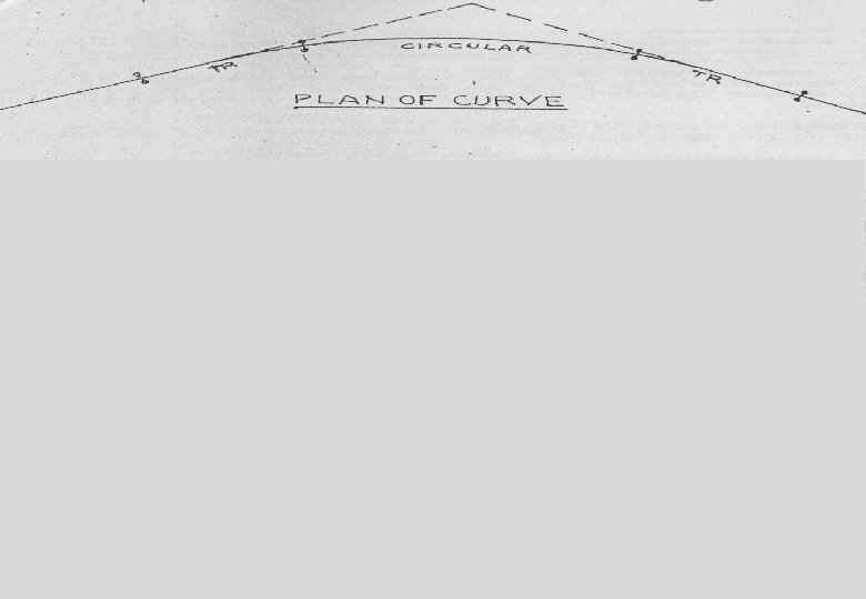
Requirements from Transition Curves • Curvature shall vary uniformly with distance – Curvature = 1/R – Versine shall vary uniformly • Cant shall vary uniformly • Transition shall be tangential to the straight as well as circular curve – Radius infinity at junction with straight – Radius R at junction with circular curve
![Transition Curves The spiral Clothoid which changes the direction angle uniformly along length Transition Curves • The spiral (Clothoid), which changes the direction angle uniformly along length,](https://slidetodoc.com/presentation_image_h2/c1a8ddc073bce1675e4bd1ae2348660b/image-6.jpg)
Transition Curves • The spiral (Clothoid), which changes the direction angle uniformly along length, is the ideal transition –i. e. L ∝ 1/R • Cubic Parabola – rate of change of curvature uniform with the distance on X direction –i. e. X ∝ 1/R
![Transition Curves There is not much difference in the layout of a spiral Transition Curves • There is not much difference in the layout of a spiral](https://slidetodoc.com/presentation_image_h2/c1a8ddc073bce1675e4bd1ae2348660b/image-7.jpg)
Transition Curves • There is not much difference in the layout of a spiral and cubic parabola until the deflection from straight is approximately 4 M and deflection angle upto 12° • On Indian Railways for Transition Curves, it is cubical parabola with the equation: Y = KX 3 (Y= X 3/6 R*L)
![Desirable Versine and Cant Diagram Cubic Parabola Curvature changes linearly v Ca Transition Desirable Versine and Cant Diagram Cubic Parabola – Curvature changes linearly v Ca Transition](https://slidetodoc.com/presentation_image_h2/c1a8ddc073bce1675e4bd1ae2348660b/image-8.jpg)
Desirable Versine and Cant Diagram Cubic Parabola – Curvature changes linearly v Ca Transition Cant variation – Linear Transition Cubic Parabola – Ease in setting/laying/maintaining
![Shift Transition Curves Inserting Transition Curves Shift Transition Curves Inserting Transition Curves](https://slidetodoc.com/presentation_image_h2/c1a8ddc073bce1675e4bd1ae2348660b/image-9.jpg)
Shift Transition Curves Inserting Transition Curves
![Shift Due to Transition Curve Circular Curve With Transition Extended Circular Curve C D Shift Due to Transition Curve Circular Curve With Transition Extended Circular Curve C D](https://slidetodoc.com/presentation_image_h2/c1a8ddc073bce1675e4bd1ae2348660b/image-10.jpg)
Shift Due to Transition Curve Circular Curve With Transition Extended Circular Curve C D Circular Curve Without Transition B E Transition Curve Tangent H S S/2 A L/2 F Shift = S = L 2/24 R L/2 G BG=L 2/6 R DE=L 2/8 R
![Length of Transition Curve Length of Transition Curve](https://slidetodoc.com/presentation_image_h2/c1a8ddc073bce1675e4bd1ae2348660b/image-11.jpg)
Length of Transition Curve
![](https://slidetodoc.com/presentation_image_h2/c1a8ddc073bce1675e4bd1ae2348660b/image-12.jpg)
![Length of Transition Curve Comfort Criteria Rate of Change of Cd RCd Length of Transition Curve • Comfort Criteria: Rate of Change of Cd (RCd) –](https://slidetodoc.com/presentation_image_h2/c1a8ddc073bce1675e4bd1ae2348660b/image-13.jpg)
Length of Transition Curve • Comfort Criteria: Rate of Change of Cd (RCd) – Rate of Change of ULA less than 0. 03 g / s taken as 0. 3 m/s 3 – Rate of Change of Cd over Transition where,
![Length of Transition Curve Comfort Criteria Rate of Change of Cd RCd Length of Transition Curve • Comfort Criteria: Rate of Change of Cd (RCd) –](https://slidetodoc.com/presentation_image_h2/c1a8ddc073bce1675e4bd1ae2348660b/image-14.jpg)
Length of Transition Curve • Comfort Criteria: Rate of Change of Cd (RCd) – Rate of Change of Cd , however, normally shall not exceed 35 mm/sec – Under Exceptional Circumstances it can be increased to 55 mm/sec
![Length of Transition Curve Comfort Criteria Rate of Change of Ca RCa Length of Transition Curve • Comfort Criteria: Rate of Change of Ca (RCa) –](https://slidetodoc.com/presentation_image_h2/c1a8ddc073bce1675e4bd1ae2348660b/image-15.jpg)
Length of Transition Curve • Comfort Criteria: Rate of Change of Ca (RCa) – For slower speeds, the actual cant causes similar comfort problems – Rate of change of Ca is just noticeable at 6575 mm/sec but normally shall not exceed 35 mm /sec – Under Exceptional Circumstances it can be increased to 55 mm /sec
![Length of Transition Curve Safety Criteria Twist Cant gradient causes twist in Length of Transition Curve • Safety Criteria (Twist) – Cant gradient causes twist in](https://slidetodoc.com/presentation_image_h2/c1a8ddc073bce1675e4bd1ae2348660b/image-16.jpg)
Length of Transition Curve • Safety Criteria (Twist) – Cant gradient causes twist in track – Critical - longest rigid wheel base – Cant gradient (i) • Limited to 1. 4 mm/m or 1 in 720 • In Exceptional Cases 2. 8 mm/M or 1 in 360 • Future Layouts with 1 in 1200
![Length of Transition Curve Length of transition will be maximum of L 1 Length of Transition Curve • Length of transition will be maximum of L 1](https://slidetodoc.com/presentation_image_h2/c1a8ddc073bce1675e4bd1ae2348660b/image-17.jpg)
Length of Transition Curve • Length of transition will be maximum of L 1 = C a * V m / R Ca or L 2 = C d * V m / R Cd or L 3 = Ca / i
![Length of Transition Curve Length of transition will be maximum of L 1 Length of Transition Curve • Length of transition will be maximum of L 1](https://slidetodoc.com/presentation_image_h2/c1a8ddc073bce1675e4bd1ae2348660b/image-18.jpg)
Length of Transition Curve • Length of transition will be maximum of L 1 = 0. 008 Ca* Vm (m, mm, kmph, RCa=35 mm/s) L 2 = 0. 008 Cd*Vm (m, mm, kmph, RCd=35 mm/s) L 3 = 0. 72 Ca (m, mm, i = 1 in 720) or or
![Length of Transition Curve In exceptional circumstances minimum length of transition will be Length of Transition Curve • In exceptional circumstances, minimum length of transition will be](https://slidetodoc.com/presentation_image_h2/c1a8ddc073bce1675e4bd1ae2348660b/image-19.jpg)
Length of Transition Curve • In exceptional circumstances, minimum length of transition will be maximum of 2/3 rd of L 1 or 2/3 rd of L 2 or ½ of L 3
![Procedure to find Speed on Curve Find equilibrium cant for the maximum speed Procedure to find Speed on Curve • Find equilibrium cant for the maximum speed](https://slidetodoc.com/presentation_image_h2/c1a8ddc073bce1675e4bd1ae2348660b/image-20.jpg)
Procedure to find Speed on Curve • Find equilibrium cant for the maximum speed – Find minimum cant required by deducting the cant deficiency from equilibrium cant • Find cant required for booked speed of goods trains. – Add cant excess and find out the maximum cant permissible • The cant to be provided shall be between the two values computed above
![Procedure to find Speed on Curve Cant to be Provided shall also be Procedure to find Speed on Curve • Cant to be Provided shall also be](https://slidetodoc.com/presentation_image_h2/c1a8ddc073bce1675e4bd1ae2348660b/image-21.jpg)
Procedure to find Speed on Curve • Cant to be Provided shall also be less than the Maximum Permissible as per IRPWM • Corresponding to actual cant provided, find maximum speed • Find out the desirable/ minimum transition length • If shift is not possible, restrict length of transition and work out cant and speed permissible corresponding to the reduced length available
![Exercise Find Maximum Permissible Speed for BG route having Speed Potential 130 Exercise Find Maximum Permissible Speed for – BG route having Speed Potential = 130](https://slidetodoc.com/presentation_image_h2/c1a8ddc073bce1675e4bd1ae2348660b/image-22.jpg)
Exercise Find Maximum Permissible Speed for – BG route having Speed Potential = 130 Kmph Rajdhani Route (Group “A”), and Degree of Curve = 2° Speed of Goods Train = 65 Kmph Cd = 100 mm and Cex = 75 mm SE = 140 mm Max. Speed = 123. 73 Kmph ≈ 120 Kmph
![Exercise Find Desirable and Minimum Transition Length for BG route having Speed Potential Exercise Find Desirable and Minimum Transition Length for – BG route having Speed Potential](https://slidetodoc.com/presentation_image_h2/c1a8ddc073bce1675e4bd1ae2348660b/image-23.jpg)
Exercise Find Desirable and Minimum Transition Length for – BG route having Speed Potential = 130 Kmph Rajdhani Route (Group “A”), and Degree of Curve = 2° Desirable Length L 1 = 134. 4 m Speed of Goods Train = 65 Kmph L = 96. 0 m Cd = 100 mm and Cex = 75 mm SE = 140 mm Max. Speed = 120 Kmph 2 L 3 = 100. 8 m Minimum Length L 1 = 89. 6 m L 2 = 64. 0 m L 3 = 50. 4 m
![Exercise Calculate Shift for BG route having Speed Potential 130 Kmph Rajdhani Exercise Calculate Shift for – BG route having Speed Potential = 130 Kmph Rajdhani](https://slidetodoc.com/presentation_image_h2/c1a8ddc073bce1675e4bd1ae2348660b/image-24.jpg)
Exercise Calculate Shift for – BG route having Speed Potential = 130 Kmph Rajdhani Route (Group “A”), and Degree of Curve = 2° Speed of Goods Train = 65 Kmph Cd = 100 mm; and Cex = 75 mm SE = 140 mm Max. Speed = 120 Kmph Desirable Length of Transition L 1 = 140 m Minimum Length of Transition L 1 = 90 m 0. 933 m and 0. 385 m
![Desirable Versine and Cant Diagram V Transition Ca Transition Desirable Versine and Cant Diagram V Transition Ca Transition](https://slidetodoc.com/presentation_image_h2/c1a8ddc073bce1675e4bd1ae2348660b/image-25.jpg)
Desirable Versine and Cant Diagram V Transition Ca Transition
![If there is no Transition Curve v Transition Ca Transition How to introduce If there is no Transition Curve ? v Transition Ca Transition How to introduce](https://slidetodoc.com/presentation_image_h2/c1a8ddc073bce1675e4bd1ae2348660b/image-26.jpg)
If there is no Transition Curve ? v Transition Ca Transition How to introduce V and Ca ?
![2 m V Virtual Transition ~2 m ? V Virtual Transition](https://slidetodoc.com/presentation_image_h2/c1a8ddc073bce1675e4bd1ae2348660b/image-27.jpg)
~2 m ? V Virtual Transition
![Virtual Transition If there is no space for transition circular curve immediately follows Virtual Transition • If there is no space for transition, circular curve immediately follows](https://slidetodoc.com/presentation_image_h2/c1a8ddc073bce1675e4bd1ae2348660b/image-28.jpg)
Virtual Transition • If there is no space for transition, circular curve immediately follows the straight, the distance between bogie centers becomes the transition virtually • For BG • For MG - 14. 6 M - 13. 7 M • Cant is provided in virtual transition length • half in straight and half in circular curve • @1 in 360 (max. cant gradient) max. cant = 14. 6 * 2. 8 = 40 mm
![Reverse and Compound Curves Reverse and Compound Curves](https://slidetodoc.com/presentation_image_h2/c1a8ddc073bce1675e4bd1ae2348660b/image-29.jpg)
Reverse and Compound Curves
![Reverse Curves Length of intermediate Transition will be Maximum of L 1 0 Reverse Curves Length of intermediate Transition will be Maximum of L 1 = 0.](https://slidetodoc.com/presentation_image_h2/c1a8ddc073bce1675e4bd1ae2348660b/image-30.jpg)
Reverse Curves Length of intermediate Transition will be Maximum of L 1 = 0. 008 * (Ca 1+Ca 2) * Vm L 2 = 0. 008 * (Cd 1+Cd 2) * Vm L 3 = 0. 72 * (Ca 1+Ca 2) Constant roll velocity during intermediate transition
![Reverse Curves For high speeds in Group A and B routes a straight Reverse Curves • For high speeds in Group A and B routes a straight](https://slidetodoc.com/presentation_image_h2/c1a8ddc073bce1675e4bd1ae2348660b/image-31.jpg)
Reverse Curves • For high speeds in Group A and B routes a straight of 50 m length shall be kept – One cycle of oscillation for passenger coach (1. 5 sec) • Otherwise, increase the transition length to eliminate the straight • If neither of the above two are possible than speed restriction of 130 KMPH on BG
![Compound Curves Compound Curves](https://slidetodoc.com/presentation_image_h2/c1a8ddc073bce1675e4bd1ae2348660b/image-32.jpg)
Compound Curves
![Compound and Reverse Curves For Compound Curves Length of Intermediate Transition shall be Compound and Reverse Curves • For Compound Curves: Length of Intermediate Transition shall be](https://slidetodoc.com/presentation_image_h2/c1a8ddc073bce1675e4bd1ae2348660b/image-33.jpg)
Compound and Reverse Curves • For Compound Curves: Length of Intermediate Transition shall be Maximum of • L 1 = 0. 008 * (Ca 1 - Ca 2) * Vm • L 2 = 0. 008 * (Cd 1 - Cd 2) * Vm • L 3 = 0. 72 * (Ca 1 - Ca 2) If length is coming less than virtual transition then common transition is deleted and the cant is run out on the length of virtual transition
![Vertical curves Vertical curves](https://slidetodoc.com/presentation_image_h2/c1a8ddc073bce1675e4bd1ae2348660b/image-34.jpg)
Vertical curves
![Types of Vertical Curves Types of Vertical Curves](https://slidetodoc.com/presentation_image_h2/c1a8ddc073bce1675e4bd1ae2348660b/image-35.jpg)
Types of Vertical Curves
![Vertical curves Vertical Curves to be provided if Algebraic Difference between the Vertical curves • Vertical Curves to be provided, if ; Algebraic Difference between the](https://slidetodoc.com/presentation_image_h2/c1a8ddc073bce1675e4bd1ae2348660b/image-36.jpg)
Vertical curves • Vertical Curves to be provided, if ; Algebraic Difference between the Grades ≥ 0. 4% (4 mm/m) • Not allowed in – Points and Crossing – Un-ballasted deck girder bridges – Transition portion of horizontal curves
![Vertical curves Important issues Vertical acceleration Drainage Sag Ventilation Summit Vertical curves • Important issues – Vertical acceleration – Drainage (Sag) – Ventilation (Summit)](https://slidetodoc.com/presentation_image_h2/c1a8ddc073bce1675e4bd1ae2348660b/image-37.jpg)
Vertical curves • Important issues – Vertical acceleration – Drainage (Sag) – Ventilation (Summit) in Tunnels ?
![Vertical curves Shall be as flat as possible to reduce Discomfort to passengers Vertical curves • Shall be as flat as possible to reduce Discomfort to passengers](https://slidetodoc.com/presentation_image_h2/c1a8ddc073bce1675e4bd1ae2348660b/image-38.jpg)
Vertical curves • Shall be as flat as possible to reduce Discomfort to passengers • Vertical Acceleration 0. 3 – 0. 45 m/s 2 2 • Radius Rv ≥ Vm / am Route A B C, D, E & MG Minimum Radius (m) 4, 000 3, 000 2, 500
![Effects of curve Curve Resistance Effects of curve: Curve Resistance](https://slidetodoc.com/presentation_image_h2/c1a8ddc073bce1675e4bd1ae2348660b/image-39.jpg)
Effects of curve: Curve Resistance
![Compensation for Curvature on gradient Known as Grade Compensation Reduction in ruling Compensation for Curvature on gradient • Known as Grade Compensation – Reduction in ruling](https://slidetodoc.com/presentation_image_h2/c1a8ddc073bce1675e4bd1ae2348660b/image-40.jpg)
Compensation for Curvature on gradient • Known as Grade Compensation – Reduction in ruling gradient • to allow for the effect of curve or – Increase in actual gradient • to get “Compensated Gradient” to get combined effect of curve + gradient • 70/R % or 0. 04% Per Degree of Curve
![Check Rails on Curves Check Rails on Curves](https://slidetodoc.com/presentation_image_h2/c1a8ddc073bce1675e4bd1ae2348660b/image-41.jpg)
Check Rails on Curves
![Check Rails on Curves CLEARANCE Too Much Wear on Outer Rail in Sharp Curves Check Rails on Curves CLEARANCE Too Much Wear on Outer Rail in Sharp Curves;](https://slidetodoc.com/presentation_image_h2/c1a8ddc073bce1675e4bd1ae2348660b/image-42.jpg)
Check Rails on Curves CLEARANCE Too Much Wear on Outer Rail in Sharp Curves; and CHECK RAIL • Para 426 of IRPWM • Clause 4, Chapter 1, BG : SOD Risk of derailment • On Curves of 8 Degrees & above • Minimum Clearance = 44 mm • Clearance = 44 + (G*-1676)/2 • G*: Actual wide gauge on the Curve • Lubrication of outer Rail for all Curves with Radius less than 600 m
![Thank You Thank You](https://slidetodoc.com/presentation_image_h2/c1a8ddc073bce1675e4bd1ae2348660b/image-43.jpg)
Thank You
![IRPWM Provisions Inspections AEN to inspect one curve in each PWI jurisdiction IRPWM Provisions • Inspections – AEN to inspect one curve in each PWI jurisdiction](https://slidetodoc.com/presentation_image_h2/c1a8ddc073bce1675e4bd1ae2348660b/image-44.jpg)
IRPWM Provisions • Inspections – AEN to inspect one curve in each PWI jurisdiction every quarter (107(4)) – PWI in-charge and his assistant shall inspect curves once in six months alternately except at group A and B routes where inspection is to be done once in four months (124(4), 139(4)) – For Concrete Sleeper track, once in six months by rotation (124 A, 139 A)
![IRPWM Provisions BG Lateral wear on Rails in Curves 301biv Group A IRPWM Provisions (BG) • Lateral wear on Rails in Curves (301(b)(iv)) – Group A](https://slidetodoc.com/presentation_image_h2/c1a8ddc073bce1675e4bd1ae2348660b/image-45.jpg)
IRPWM Provisions (BG) • Lateral wear on Rails in Curves (301(b)(iv)) – Group A and B : 8 mm – Group C and D : 10 mm • Minimising wear on outer Rail (427(2)) – Rail flange lubricators shall be provided in curves less than 600 m radius – First one shall be ahead of the curve
![IRPWM Provisions BG Cut in rails in SWR track 424 To make IRPWM Provisions (BG) • Cut in rails in SWR track (424) – To make](https://slidetodoc.com/presentation_image_h2/c1a8ddc073bce1675e4bd1ae2348660b/image-46.jpg)
IRPWM Provisions (BG) • Cut in rails in SWR track (424) – To make the joints square when the gain of inner rail becomes equal to pitch of the first bolt hole – Gain of inner rail given by: d= LG/R, L is length of curve. • On curves less than 400 m radius, the joints shall be laid staggered
![IRPWM Provisions BG After relaying On curves Versine variation over Theoretical versine on IRPWM Provisions (BG) After relaying • On curves, Versine variation over Theoretical versine on](https://slidetodoc.com/presentation_image_h2/c1a8ddc073bce1675e4bd1ae2348660b/image-47.jpg)
IRPWM Provisions (BG) After relaying • On curves, Versine variation over Theoretical versine on 20 m chord (316) – 600 m radius and more – Less than 600 m radius : 5 mm : 10 mm • Gauge in Track on curves (403(1)) – More than 350 m radius : -5 mm to + 3 mm – Less than 350 m radius : upto +10 mm
![IRPWM Provisions BG Inservice Gauge 2242ev On straight 6 mm IRPWM Provisions (BG) In-service • Gauge (224(2)(e)(v)) – On straight : (-) 6 mm](https://slidetodoc.com/presentation_image_h2/c1a8ddc073bce1675e4bd1ae2348660b/image-48.jpg)
IRPWM Provisions (BG) In-service • Gauge (224(2)(e)(v)) – On straight : (-) 6 mm to (+) 6 mm – On Curves with radius 440 m or more: (-) 6 mm to (+) 15 mm – On curves radius less than 440 m: upto (+) 20 mm
![IRPWM Provisions BG Inservice tolerances speed 100 kmph 140 kmph Twist 6072iii IRPWM Provisions (BG) In-service tolerances (speed >100 kmph, <140 kmph) • Twist (607(2)(iii)) –](https://slidetodoc.com/presentation_image_h2/c1a8ddc073bce1675e4bd1ae2348660b/image-49.jpg)
IRPWM Provisions (BG) In-service tolerances (speed >100 kmph, <140 kmph) • Twist (607(2)(iii)) – On straight/curves • Upto 2 mm/M • At Isolated Locations : upto 3. 5 mm/M – On transitions • Upto 1 mm/M • At Isolated Locations : upto 2. 1 mm/M
![IRPWM Provisions BG Inservice tolerances speed 100 kmph 140 kmph Alignment defect 6072i IRPWM Provisions (BG) In-service tolerances (speed >100 kmph, <140 kmph) • Alignment defect (607(2)(i))](https://slidetodoc.com/presentation_image_h2/c1a8ddc073bce1675e4bd1ae2348660b/image-50.jpg)
IRPWM Provisions (BG) In-service tolerances (speed >100 kmph, <140 kmph) • Alignment defect (607(2)(i)) on 7. 5 m chord – On straight • Upto 5 mm • At Isolated Locations : upto 10 mm – On curves • Upto ± 5 mm over average versine • At Isolated locations upto ± 7 mm over average versine • Chord to chord ≤ 10 mm
![IRPWM Provisions Radius of curve 4011 R 125C 2V For measuring IRPWM Provisions • Radius of curve (401(1)) R = 125*C 2/V • For measuring](https://slidetodoc.com/presentation_image_h2/c1a8ddc073bce1675e4bd1ae2348660b/image-51.jpg)
IRPWM Provisions • Radius of curve (401(1)) R = 125*C 2/V • For measuring versine (401(3)) – Normal: • 20 m chord overlapping with stations at 10 m – P & Cs: (for lead and turn-in curve) • 6 m chord overlapping with stations at 1. 5 m (This shall be 3 m as per para 237 (4) (b) and (c) of IRPWM)
![IRPWM Provisions Safe speed on a Curve 4051a V 0 27 R IRPWM Provisions • Safe speed on a Curve (405(1)(a)) V = 0. 27 √{R](https://slidetodoc.com/presentation_image_h2/c1a8ddc073bce1675e4bd1ae2348660b/image-52.jpg)
IRPWM Provisions • Safe speed on a Curve (405(1)(a)) V = 0. 27 √{R (Ca + Cd)} • Non transitioned Curve (405(2)(a)) Length of virtual transition : 14. 6 m • Inner rail is taken as reference; and outer rail is raised by amount of superelevation (402)
![IRPWM Provisions Curve boards4091 Curve board shall be provided at tangent point IRPWM Provisions • Curve boards(409(1)) – Curve board shall be provided at tangent point](https://slidetodoc.com/presentation_image_h2/c1a8ddc073bce1675e4bd1ae2348660b/image-53.jpg)
IRPWM Provisions • Curve boards(409(1)) – Curve board shall be provided at tangent point on outside of the curve • Curve posts (409(2)) – Rail posts indicating beginning and end of transition, painted red and white respectively shall be provided (at beginning/end of virtual transition of nontransitioned curves).
![Curve Board Curve Board](https://slidetodoc.com/presentation_image_h2/c1a8ddc073bce1675e4bd1ae2348660b/image-54.jpg)
Curve Board
![IRPWM Provisions Superelevation marking on rails 4093 Value of superelevation shall be IRPWM Provisions • Super-elevation marking on rails (409(3)) – Value of super-elevation shall be](https://slidetodoc.com/presentation_image_h2/c1a8ddc073bce1675e4bd1ae2348660b/image-55.jpg)
IRPWM Provisions • Super-elevation marking on rails (409(3)) – Value of super-elevation shall be marked on the inside face of the web of inner rail at every versine stations in transition portion – Value of cant as above shall be marked at the beginning and end of the circular curve – For longer curves, the value of super-elevation shall be repeated as above at intervals not exceeding 250 m
![Lead Curve following Turnout Minimum radius of lead curve 4102 350 m Lead Curve following Turnout • Minimum radius of lead curve (410(2)) : 350 m](https://slidetodoc.com/presentation_image_h2/c1a8ddc073bce1675e4bd1ae2348660b/image-56.jpg)
Lead Curve following Turnout • Minimum radius of lead curve (410(2)) : 350 m • Minimum radius of turn in curves : 220 m in exceptional circumstances (with PSC/ST sleepers and full ML ballast profile) • There shall be no change in super-elevation 20 m on either side of the toe of switch and nose of crossing (412) • Turnout followed by reverse curve, change in cant behind crossing is permitted. Cant limited to 65 mm, run out at 2. 8 mm/m (414(2))
![Lead portion and Turnin curves The variation in versine on two successive stations in Lead portion and Turn-in curves The variation in versine on two successive stations in](https://slidetodoc.com/presentation_image_h2/c1a8ddc073bce1675e4bd1ae2348660b/image-57.jpg)
Lead portion and Turn-in curves The variation in versine on two successive stations in lead curve and turn in curve portions should not be more than 4 mm; and versine at each station should also not be beyond ± 3 mm. from its designed value (IRPWM Para 237(4)(d))
![Thank You Thank You](https://slidetodoc.com/presentation_image_h2/c1a8ddc073bce1675e4bd1ae2348660b/image-58.jpg)
Thank You
![Extra Clearances on curves Lean and Sway Extra Clearances on curves Lean and Sway](https://slidetodoc.com/presentation_image_h2/c1a8ddc073bce1675e4bd1ae2348660b/image-59.jpg)
Extra Clearances on curves Lean and Sway
![Clearances on curves Lean L H CaG H height of Clearances on curves : Lean L = H * Ca/G H = height of](https://slidetodoc.com/presentation_image_h2/c1a8ddc073bce1675e4bd1ae2348660b/image-60.jpg)
Clearances on curves : Lean L = H * Ca/G H = height of the structure or maximum height of vehicle whichever is less
![Clearances on curves Additional Allowance due to Lurch Sway Inside of Clearances on curves : Additional Allowance due to Lurch & Sway • Inside of](https://slidetodoc.com/presentation_image_h2/c1a8ddc073bce1675e4bd1ae2348660b/image-61.jpg)
Clearances on curves : Additional Allowance due to Lurch & Sway • Inside of a Curve – ¼ of lean due to super-elevation • Outside of a Curve – Not to be considered if lean is there • We do not take advantage of the extra clearance given by lean away from outer side structures
![Extra Clearances on Curves Platforms and structures Extra Clearances on Curves: Platforms and structures](https://slidetodoc.com/presentation_image_h2/c1a8ddc073bce1675e4bd1ae2348660b/image-62.jpg)
Extra Clearances on Curves: Platforms and structures
![Clearance On Curves Effect of Chords Clearance On Curves : Effect of Chords](https://slidetodoc.com/presentation_image_h2/c1a8ddc073bce1675e4bd1ae2348660b/image-63.jpg)
Clearance On Curves : Effect of Chords
![OverThrow and EndThrow on Curves Vo14 78528R Over Throw Vo 14 785 m 21 Over-Throw and End-Throw on Curves Vo=14. 7852/8*R Over Throw (Vo) 14. 785 m 21.](https://slidetodoc.com/presentation_image_h2/c1a8ddc073bce1675e4bd1ae2348660b/image-64.jpg)
Over-Throw and End-Throw on Curves Vo=14. 7852/8*R Over Throw (Vo) 14. 785 m 21. 340 m End Throw (VE) VE=(21. 342 -14. 7852)/8*R
![Extra Clearances due to Curvatures Platforms structures Inside of curve VO Extra Clearances due to Curvatures • Platforms/ structures – Inside of curve • (VO](https://slidetodoc.com/presentation_image_h2/c1a8ddc073bce1675e4bd1ae2348660b/image-65.jpg)
Extra Clearances due to Curvatures • Platforms/ structures – Inside of curve • (VO + L + S - 51) mm – Outside of curve • (VE – 25) mm
![Extra Clearances on Curved Parallel Tracks Extra Clearances on Curved Parallel Tracks](https://slidetodoc.com/presentation_image_h2/c1a8ddc073bce1675e4bd1ae2348660b/image-66.jpg)
Extra Clearances on Curved Parallel Tracks
![Extra Clearances due to Curvatures Between Adjacent Tracks VO VE 2 Extra Clearances due to Curvatures • Between Adjacent Tracks VO + VE + 2](https://slidetodoc.com/presentation_image_h2/c1a8ddc073bce1675e4bd1ae2348660b/image-67.jpg)
Extra Clearances due to Curvatures • Between Adjacent Tracks VO + VE + 2 * (L/4) • In new works, if c/c track is 5300 mm, extra clearance is to be provided for curves beyond 5° only.
![Thank You Thank You](https://slidetodoc.com/presentation_image_h2/c1a8ddc073bce1675e4bd1ae2348660b/image-68.jpg)
Thank You
![Turnouts taking off from curve Turnouts taking off from curve](https://slidetodoc.com/presentation_image_h2/c1a8ddc073bce1675e4bd1ae2348660b/image-69.jpg)
Turnouts taking off from curve
![Turnouts taking off from curve Straight Main Line Curved main Line Re Rs R Turnouts taking off from curve Straight Main Line Curved main Line Re Rs R](https://slidetodoc.com/presentation_image_h2/c1a8ddc073bce1675e4bd1ae2348660b/image-70.jpg)
Turnouts taking off from curve Straight Main Line Curved main Line Re Rs R Rm
![Turnouts on Curves Similar Flexure ML TO Contrary Flexure ML 74 Turnouts on Curves Similar Flexure ML T/O Contrary Flexure ML 74](https://slidetodoc.com/presentation_image_h2/c1a8ddc073bce1675e4bd1ae2348660b/image-71.jpg)
Turnouts on Curves Similar Flexure ML T/O Contrary Flexure ML 74
![Resultant Lead Radius in Similar Flexure Turnouts Main line with Radius R 1 and Resultant Lead Radius in Similar Flexure Turnouts Main line with Radius R 1 and](https://slidetodoc.com/presentation_image_h2/c1a8ddc073bce1675e4bd1ae2348660b/image-72.jpg)
Resultant Lead Radius in Similar Flexure Turnouts Main line with Radius R 1 and Degree D 1 Turnout Laid on Straight Lead curve with Radius R & Degree D Lead curve with resultant Radius R 2 & resultant Degree D 2 For similar flexure, D 2 = D 1 + D 1750/R 2 = 1750/R 1 + 1750/R 1/R 2= 1/R 1 + 1/R 75
![Resultant Lead Radius in Contrary Flexure Turnouts Main line with Radius R 1 and Resultant Lead Radius in Contrary Flexure Turnouts Main line with Radius R 1 and](https://slidetodoc.com/presentation_image_h2/c1a8ddc073bce1675e4bd1ae2348660b/image-73.jpg)
Resultant Lead Radius in Contrary Flexure Turnouts Main line with Radius R 1 and Degree D 1 Turnout Laid on Straight Lead curve with radius R & degree D For contrary flexure, D 2 = D 1 - D, 1750/R 2 = 1750/R 1 - 1750/R, 1/R 2= 1/R 1 - 1/R Lead curve with resultant Radius R 2 & resultant Degree D 2 76
![](https://slidetodoc.com/presentation_image_h2/c1a8ddc073bce1675e4bd1ae2348660b/image-74.jpg)
![Equivalent Curvature The train moving on the turnout side experiences dual curvature Equivalent Curvature • The train moving on the turnout side experiences dual curvature •](https://slidetodoc.com/presentation_image_h2/c1a8ddc073bce1675e4bd1ae2348660b/image-75.jpg)
Equivalent Curvature • The train moving on the turnout side experiences dual curvature • Due to the main line curve • Due to the turnout itself • The curvatures get added up • Curvature=1/Radius
![Turnouts in Similar Flexure ReRmRsRmRs Re Equivalent Radius Rm Main Line Radius Rs Switch Turnouts in Similar Flexure Re=Rm*Rs/(Rm+Rs) Re: Equivalent Radius Rm: Main Line Radius Rs: Switch](https://slidetodoc.com/presentation_image_h2/c1a8ddc073bce1675e4bd1ae2348660b/image-76.jpg)
Turnouts in Similar Flexure Re=Rm*Rs/(Rm+Rs) Re: Equivalent Radius Rm: Main Line Radius Rs: Switch Radius
![Turnouts in Contrary Flexure ReRmRsRmRs Re Equivalent Radius Rm Main Line Radius Rs Switch Turnouts in Contrary Flexure Re=Rm*Rs/(Rm-Rs) Re: Equivalent Radius Rm: Main Line Radius Rs: Switch](https://slidetodoc.com/presentation_image_h2/c1a8ddc073bce1675e4bd1ae2348660b/image-77.jpg)
Turnouts in Contrary Flexure Re=Rm*Rs/(Rm-Rs) Re: Equivalent Radius Rm: Main Line Radius Rs: Switch Radius
![Speed on Curve having Turnouts Trains move on main line as well as Speed on Curve having Turnouts • Trains move on main line as well as](https://slidetodoc.com/presentation_image_h2/c1a8ddc073bce1675e4bd1ae2348660b/image-78.jpg)
Speed on Curve having Turnouts • Trains move on main line as well as the turnout side • Allowable cant to be found after checking for both the tracks • Similar flexure: turnout side train moves with slower speed and more cant is there on main line so check for cant excess • Contrary flexure: Turnout side train with Negative cant. Check for cant deficiency
![Calculation of Cant Similar flexure Turnout Calculate equilibrium super elevation for turnout Calculation of Cant • Similar flexure Turnout: – Calculate equilibrium super elevation for turnout](https://slidetodoc.com/presentation_image_h2/c1a8ddc073bce1675e4bd1ae2348660b/image-79.jpg)
Calculation of Cant • Similar flexure Turnout: – Calculate equilibrium super elevation for turnout side as per maximum speed permitted on turnout side (i. e. Ceqto) Ceqto = GV 2/127 Rto (Rto is the resultant radius of Lead curve) – Add 75 mm of cant excess, this is the super elevation which can be provided on turnout side (i. e. Ca). Ca = Ceqto + 75 mm – Speed for main line can be calculated by taking Ca as calculated above and taking Cd as 75 mm. Ca + Cd = GV 2/127 Rm ML T/O
![Calculation of Cant TO Contrary flexure Calculate equilibrium super elevation for turnout side Calculation of Cant T/O • Contrary flexure– Calculate equilibrium super elevation for turnout side](https://slidetodoc.com/presentation_image_h2/c1a8ddc073bce1675e4bd1ae2348660b/image-80.jpg)
Calculation of Cant T/O • Contrary flexure– Calculate equilibrium super elevation for turnout side as per maximum speed permitted on turnout side (i. e. Ceqto) Ceqto = GV 2/127 Rto (Rto is the resultant radius of Lead curve) – Deduct it from 75 mm i. e. cant deficiency, this is the super elevation which can be provided on main line (i. e. Ca) Ca =75 mm - Ceqto – Speed for main line can be calculated by taking Ca as calculated above and taking Cd as 75 mm. Ca + Cd = GV 2/127 Rm ML
![Turnouts in Contrary Flexure Curves of contrary flexure Equilibrium super elevation for Turnouts in Contrary Flexure • Curves of contrary flexure – Equilibrium super elevation for](https://slidetodoc.com/presentation_image_h2/c1a8ddc073bce1675e4bd1ae2348660b/image-81.jpg)
Turnouts in Contrary Flexure • Curves of contrary flexure – Equilibrium super elevation for turnout side C = G * V 2 / (127 R) $ V: Speed in KPMH for Turnout, R: Metres, C: mm, G: mm – Super-elevation For Main Line (Negative Super-elevation For Turnout) is 75 - C ($ The old formula in SOD has been revised in CS No. 3)
![Thank You Thank You](https://slidetodoc.com/presentation_image_h2/c1a8ddc073bce1675e4bd1ae2348660b/image-82.jpg)
Thank You
Affirmative easement
Prescriptive easement pennsylvania
Non possessory interest
Partial interest
General lien vs specific lien
Cant deficiency in railway formula
Package diagram for railway reservation system
Through packing of railway track
Fisher v bell literal rule
Afres full form in railway
Ryder v wombwell
Geometric design of railway
Destressing temperature
Fan shaped layout
Usfd machine in railway
Trans-siberian railway
Crs sanction in railway
Diamond crossing with double slip
Mild steel canted bearing plate
Cant excess
Object controller signalling
Irpsm login
Long welded rail
Elastic fastening in railway
Hot weather patrolling in railway
Copy
Sej gap measurement
Blanketing material
019 standard
Railway discipline and appeal rules book
Modern railway systems
Advantages of the mischief rule
Contrary flexure
Railway station classification
Heel clearance in railway
Transsiberian railroad
Pot sleepers
Pacific railway act
Lwr and cwr
Cenelec railway standards
Nencki dämpferprüfpresse ndt
Rdso guidelines for earthwork
Mfi machine in railway full form
Function of ict
Improved sej
Lesson plan for from a railway carriage
Indian railway small track machine manual
Irwcms training
Motor trolly
Trolley refuge dimension
Way leave facility
Mbse rail
Wderf
Alberni pacific railway
Railway land licensing circular
Railway engineering
Hot weather patrolling in railway
Double cutting in railway signalling
Railway network sweden
Dolleys
Indian railways track machine manual
Brachistochrone
The secondary winding of a pth
Nelson curve
Msn quiz
18 curves com
Plotting curves in matlab
Learning curves 2003
Fills in gaps in data and fit data into curves
Creating production possibilities schedules and curves
Grafik koordinat kutub
Heating cooling curve
Different types of frequency curves
Fractal curve in computer graphics
Convex mirror uses
The sine and cosine curves intersect infinitely
The asymptote parallel to x-axis is obtained by equating
Elee curves
Engineering drawing curves
Heating curve
Curves of intersection in engineering drawing
Why do titration curves flatten out
Physical behavior of matter heating and cooling curves