UNIT5 Curves and Surfaces Curves Curves are one

UNIT-5 Curves and Surfaces

Curves • Curves are one dimensional entities where the function is nonlinear Curves 2

Curves • • Modeling computer graphics element with curves requires specialized handles that manage the look of a curve in an intuitive way In addition, seaming curves to build models is also important, for example changing complexity in the middle of a curve (Maya makes it trivial) 3

Representations for curves • Parametric representation x = x(u), y = y(u) or simply p(u) where p = x y More robust and general than other forms Gives better control over curves and surfaces Notation: p(u) = c 0 + c 1 u + c 2 u 2 cix where each c is a vector, ci = ciy 4

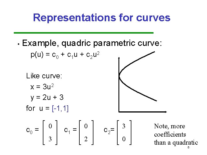
Representations for curves • Example, quadric parametric curve: p(u) = c 0 + c 1 u + c 2 u 2 Like curve: x = 3 u 2 y = 2 u + 3 for u = [ 1, 1] c 0 = 0 3 c 1 = 0 2 c 2= 3 0 Note, more coefficients than a quadratic 5

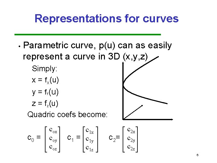
Representations for curves • Parametric curve, p(u) can as easily represent a curve in 3 D (x, y, z) Simply: x = fx(u) y = fy(u) z = fz(u) Quadric coefs become: c 0 = cox coy coz c 1 x c 1 = c 1 y c 1 z c 2 x c 2= c 2 y c 2 z 6

Parametric Cubic (pc) curves Extension of quadrics to cubics • Represented as: p(u) = c 0 + c 1 u + c 2 u 2 + c 3 u 3 • • Also called Hermite curves after the 17 th century mathematician 7

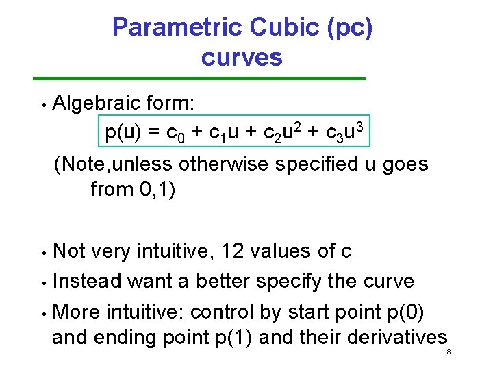
Parametric Cubic (pc) curves • Algebraic form: p(u) = c 0 + c 1 u + c 2 u 2 + c 3 u 3 (Note, unless otherwise specified u goes from 0, 1) Not very intuitive, 12 values of c • Instead want a better specify the curve • More intuitive: control by start point p(0) and ending point p(1) and their derivatives • 8

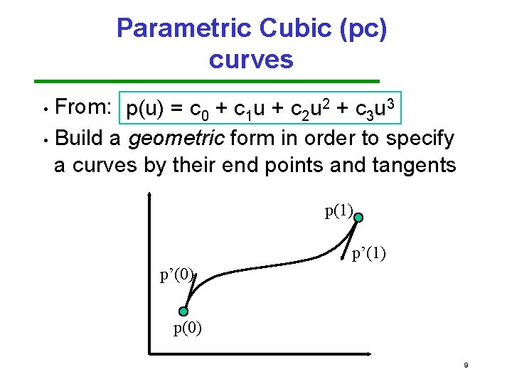
Parametric Cubic (pc) curves From: p(u) = c 0 + c 1 u + c 2 u 2 + c 3 u 3 • Build a geometric form in order to specify a curves by their end points and tangents • p(1) p’(0) p(0) 9

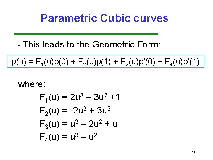
Parametric Cubic curves • This leads to the Geometric Form: p(u) = F 1(u)p(0) + F 2(u)p(1) + F 3(u)p’(0) + F 4(u)p’(1) where: F 1(u) = 2 u 3 – 3 u 2 +1 F 2(u) = 2 u 3 + 3 u 2 F 3(u) = u 3 – 2 u 2 + u F 4(u) = u 3 – u 2 10

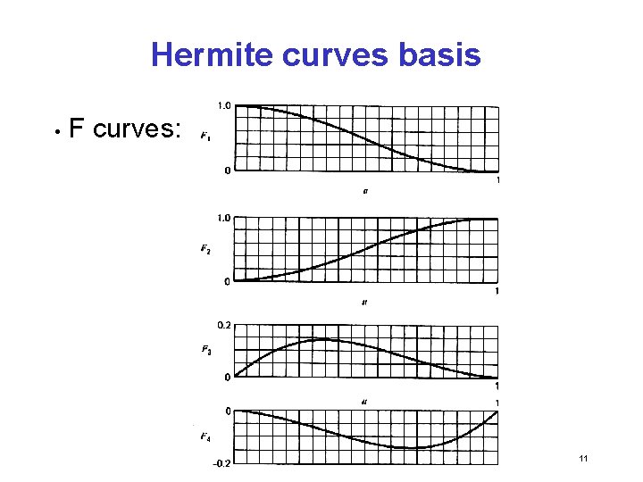
Hermite curves basis • F curves: 11

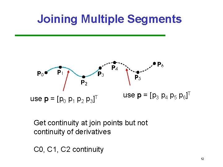
Joining Multiple Segments use p = [p 0 p 1 p 2 p 3 ]T use p = [p 3 p 4 p 5 p 6]T Get continuity at join points but not continuity of derivatives C 0, C 1, C 2 continuity 12

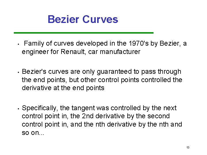
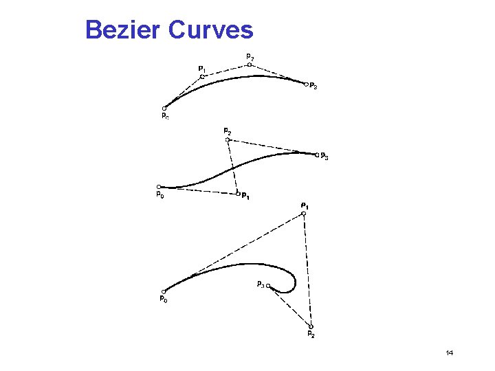
Bezier Curves • • • Family of curves developed in the 1970's by Bezier, a engineer for Renault, car manufacturer Bezier's curves are only guaranteed to pass through the end points, but other control points controlled the derivative at the end points Specifically, the tangent was controlled by the next control point in, the 2 nd derivative by the second control point in, and the nth derivative by the nth and so on. . . 13

Bezier Curves 14

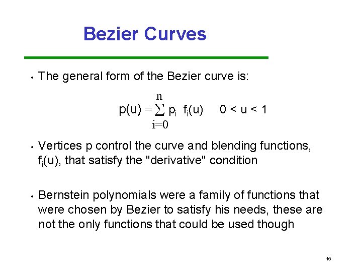
Bezier Curves • The general form of the Bezier curve is: n p(u) = S pi fi(u) 0<u<1 i=0 • • Vertices p control the curve and blending functions, fi(u), that satisfy the "derivative" condition Bernstein polynomials were a family of functions that were chosen by Bezier to satisfy his needs, these are not the only functions that could be used though 15

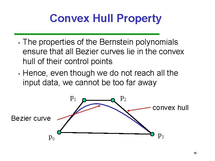
Convex Hull Property • • The properties of the Bernstein polynomials ensure that all Bezier curves lie in the convex hull of their control points Hence, even though we do not reach all the input data, we cannot be too far away p 1 p 2 convex hull Bezier curve p 0 p 3 16

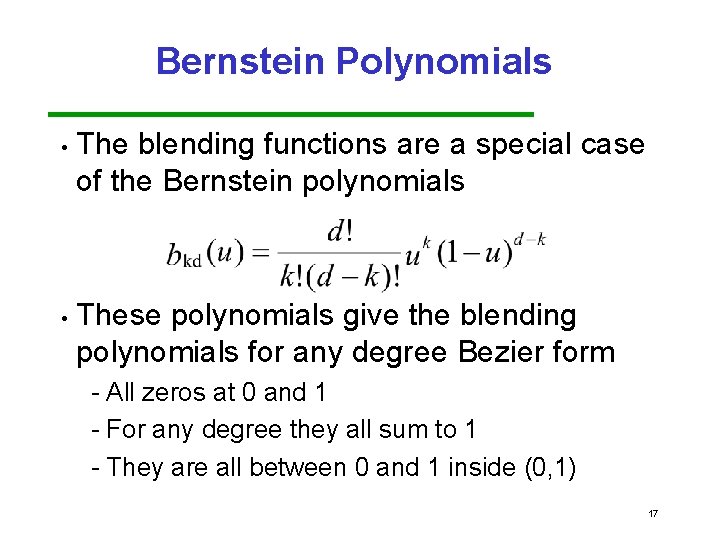
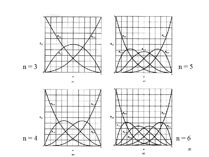
Bernstein Polynomials • • The blending functions are a special case of the Bernstein polynomials These polynomials give the blending polynomials for any degree Bezier form All zeros at 0 and 1 For any degree they all sum to 1 They are all between 0 and 1 inside (0, 1) 17

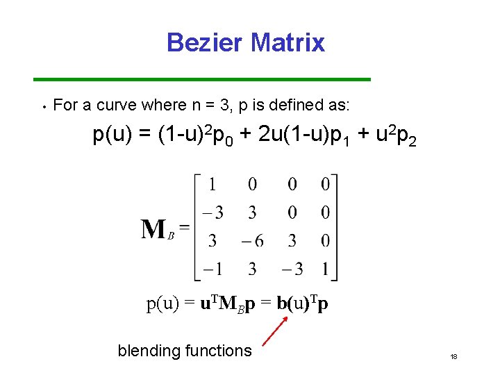
Bezier Matrix • For a curve where n = 3, p is defined as: p(u) = (1 u)2 p 0 + 2 u(1 u)p 1 + u 2 p 2 p(u) = u. TMBp = b(u)Tp blending functions 18

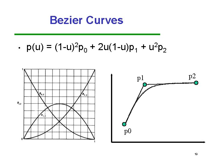
Bezier Curves • p(u) = (1 u)2 p 0 + 2 u(1 u)p 1 + u 2 p 2 p 1 p 2 p 0 19

n=3 n=4 n=5 n=6 20

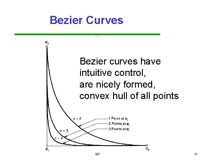
Bezier Curves Bezier curves have intuitive control, are nicely formed, convex hull of all points 21

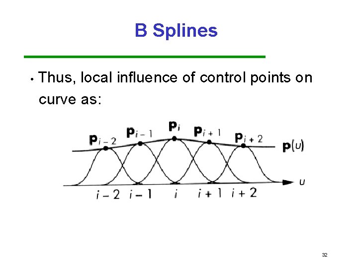
B Splines One problem with the curves we have looked at is that changing a single control point affects the whole curve (this is called global propogation, ) • Also, depends on # of control pts • B Splines offer an alternative, to only affect the local region if a single control point is modified (i. e. local propogation) • 22

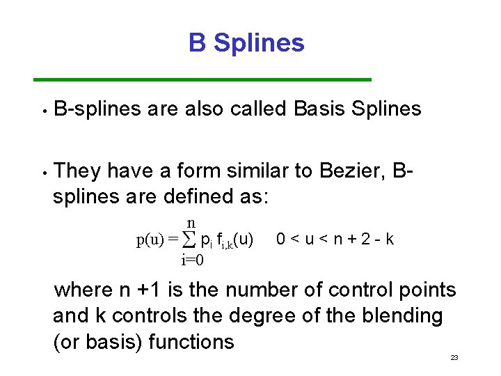
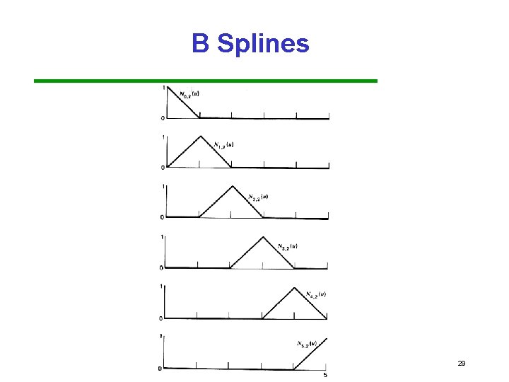
B Splines • • B splines are also called Basis Splines They have a form similar to Bezier, B splines are defined as: n p(u) = S pi fi, k(u) i=0 0<u<n+2 k where n +1 is the number of control points and k controls the degree of the blending (or basis) functions 23

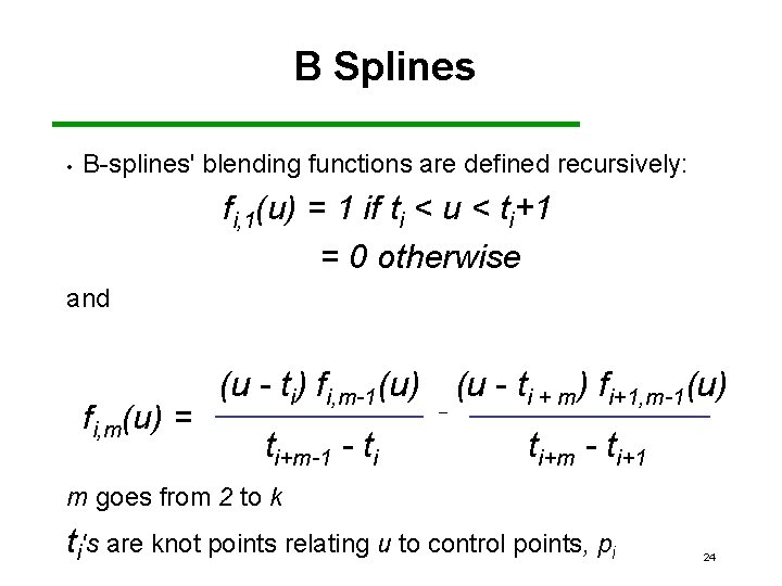
B Splines • B splines' blending functions are defined recursively: fi, 1(u) = 1 if ti < u < ti+1 = 0 otherwise and fi, m(u) = (u - ti) fi, m-1(u) ti+m-1 - ti _ (u - ti + m) fi+1, m-1(u) ti+m - ti+1 m goes from 2 to k ti's are knot points relating u to control points, pi 24

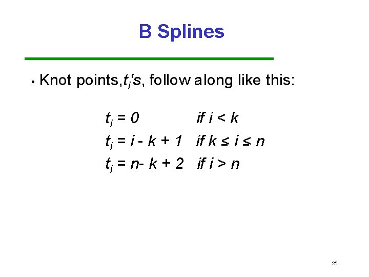
B Splines • Knot points, ti's, follow along like this: ti = 0 if i < k ti = i - k + 1 if k < i < n ti = n- k + 2 if i > n 25

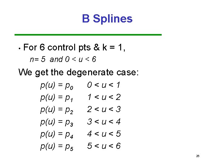
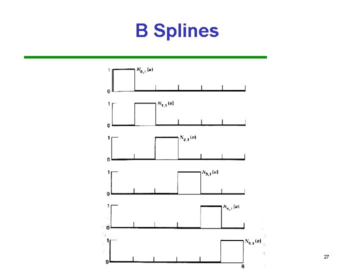
B Splines • For 6 control pts & k = 1, n= 5 and 0 < u < 6 We get the degenerate case: p(u) = p 0 p(u) = p 1 p(u) = p 2 p(u) = p 3 p(u) = p 4 p(u) = p 5 0<u<1 1<u<2 2<u<3 3<u<4 4<u<5 5<u<6 26

B Splines 27

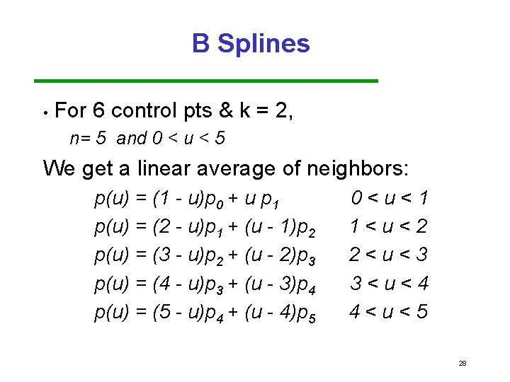
B Splines • For 6 control pts & k = 2, n= 5 and 0 < u < 5 We get a linear average of neighbors: p(u) = (1 - u)p 0 + u p 1 p(u) = (2 - u)p 1 + (u - 1)p 2 p(u) = (3 - u)p 2 + (u - 2)p 3 p(u) = (4 - u)p 3 + (u - 3)p 4 p(u) = (5 - u)p 4 + (u - 4)p 5 0<u<1 1<u<2 2<u<3 3<u<4 4<u<5 28

B Splines 29

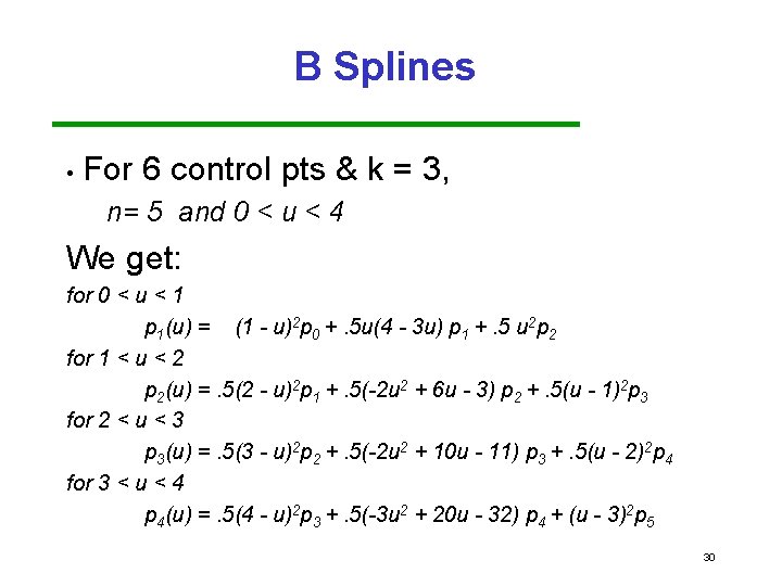
B Splines • For 6 control pts & k = 3, n= 5 and 0 < u < 4 We get: for 0 < u < 1 p 1(u) = (1 - u)2 p 0 +. 5 u(4 - 3 u) p 1 +. 5 u 2 p 2 for 1 < u < 2 p 2(u) =. 5(2 - u)2 p 1 +. 5(-2 u 2 + 6 u - 3) p 2 +. 5(u - 1)2 p 3 for 2 < u < 3 p 3(u) =. 5(3 - u)2 p 2 +. 5(-2 u 2 + 10 u - 11) p 3 +. 5(u - 2)2 p 4 for 3 < u < 4 p 4(u) =. 5(4 - u)2 p 3 +. 5(-3 u 2 + 20 u - 32) p 4 + (u - 3)2 p 5 30

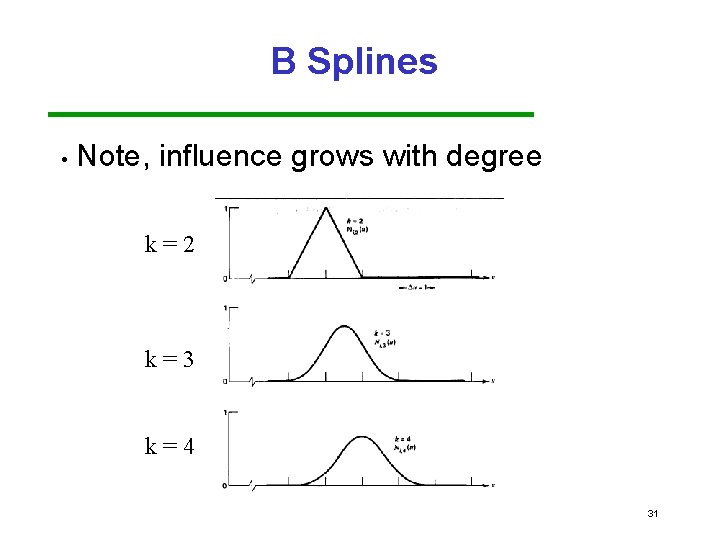
B Splines • Note, influence grows with degree k=2 k=3 k=4 31

B Splines • Thus, local influence of control points on curve as: 32

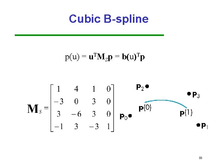
Cubic B-spline p(u) = u. TMSp = b(u)Tp 33

Curves vs. Surfaces Curves are one dimensional entities where the function is nonlinear • Surfaces are formed from two dimensional functions • Linear functions give planes and polygons y Curves x z Surfaces 34

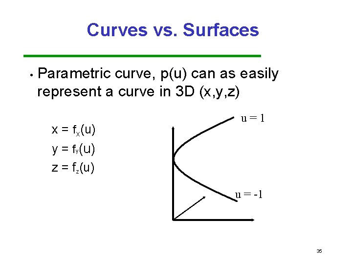
Curves vs. Surfaces • Parametric curve, p(u) can as easily represent a curve in 3 D (x, y, z) x = fx(u) u=1 y = fy(u) z = fz(u) u = -1 35

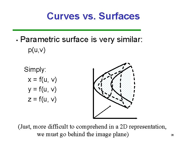
Curves vs. Surfaces • Parametric surface is very similar: p(u, v) Simply: x = f(u, v) y = f(u, v) z = f(u, v) (Just, more difficult to comprehend in a 2 D representation, we must go behind the image plane) 36

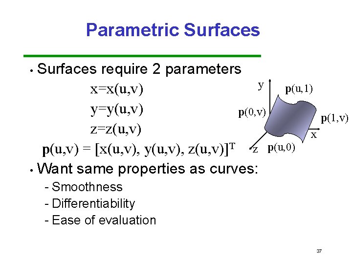
Parametric Surfaces require 2 parameters y p(u, 1) x=x(u, v) y=y(u, v) p(0, v) p(1, v) z=z(u, v) x p(u, v) = [x(u, v), y(u, v), z(u, v)]T z p(u, 0) • Want same properties as curves: • Smoothness Differentiability Ease of evaluation 37

Bezier Patches Using same data array P=[pij] as with interpolating form Patch lies in convex hull 38

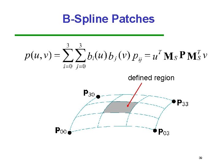
B-Spline Patches defined region 39

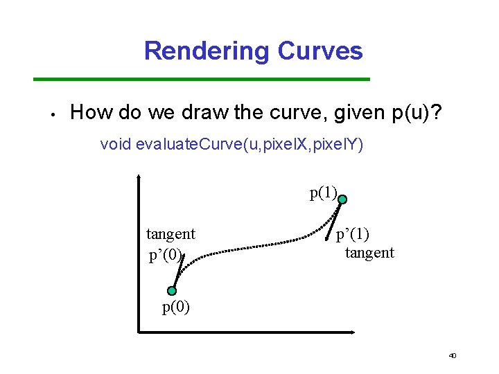
Rendering Curves • How do we draw the curve, given p(u)? void evaluate. Curve(u, pixel. X, pixel. Y) p(1) tangent p’(0) p’(1) tangent p(0) 40

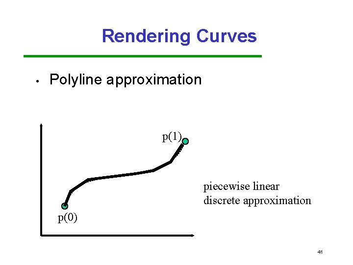
Rendering Curves • Polyline approximation p(1) piecewise linear discrete approximation p(0) 41

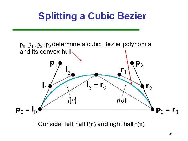
Splitting a Cubic Bezier p 0, p 1 , p 2 , p 3 determine a cubic Bezier polynomial and its convex hull Consider left half l(u) and right half r(u) 42

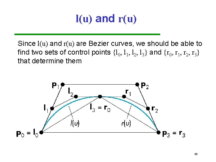
l(u) and r(u) Since l(u) and r(u) are Bezier curves, we should be able to find two sets of control points {l 0, l 1, l 2, l 3} and {r 0, r 1, r 2, r 3} that determine them 43

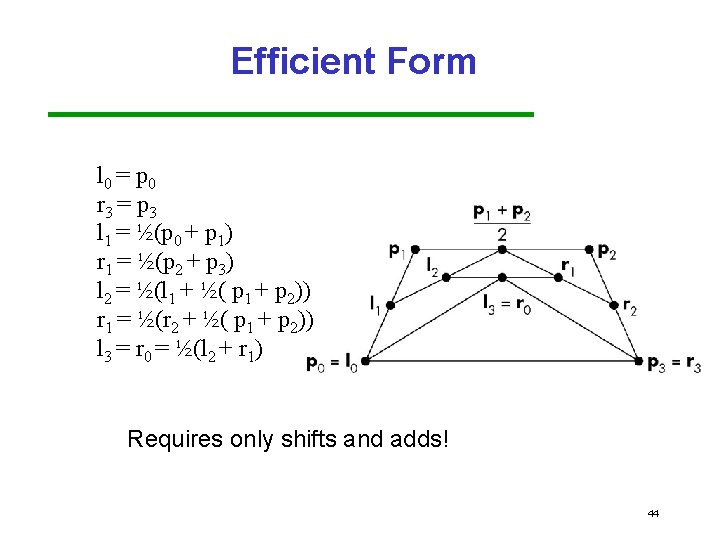
Efficient Form l 0 = p 0 r 3 = p 3 l 1 = ½(p 0 + p 1) r 1 = ½(p 2 + p 3) l 2 = ½(l 1 + ½( p 1 + p 2)) r 1 = ½(r 2 + ½( p 1 + p 2)) l 3 = r 0 = ½(l 2 + r 1) Requires only shifts and adds! 44

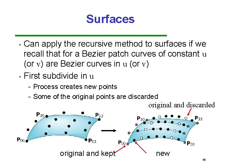
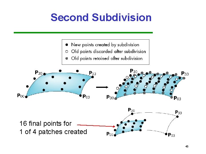
Surfaces • • Can apply the recursive method to surfaces if we recall that for a Bezier patch curves of constant u (or v) are Bezier curves in u (or v) First subdivide in u Process creates new points Some of the original points are discarded original and kept new 45

Second Subdivision 16 final points for 1 of 4 patches created 46

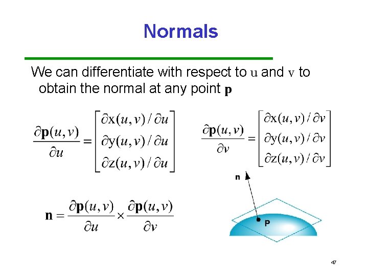
Normals We can differentiate with respect to u and v to obtain the normal at any point p 47

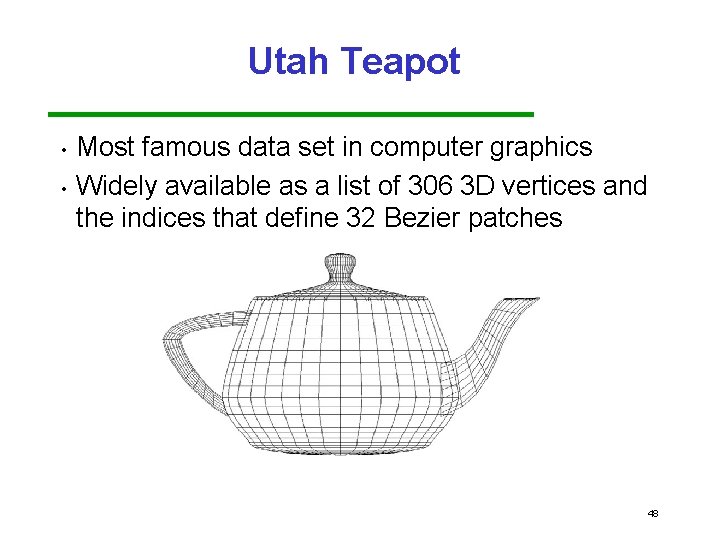
Utah Teapot • • Most famous data set in computer graphics Widely available as a list of 306 3 D vertices and the indices that define 32 Bezier patches 48