Phylogentic Tree Construction Lecture for CS 498 CXZ

Phylogentic Tree Construction (Lecture for CS 498 -CXZ Algorithms in Bioinformatics) Nov. 29, 2005 Cheng. Xiang Zhai Department of Computer Science University of Illinois, Urbana-Champaign

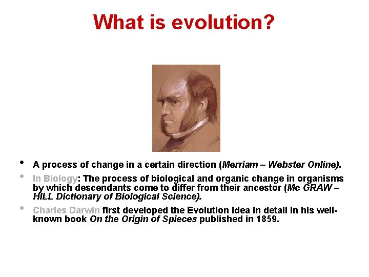
What is evolution? • • • A process of change in a certain direction (Merriam – Webster Online). In Biology: The process of biological and organic change in organisms by which descendants come to differ from their ancestor (Mc GRAW – HILL Dictionary of Biological Science). Charles Darwin first developed the Evolution idea in detail in his wellknown book On the Origin of Spieces published in 1859.

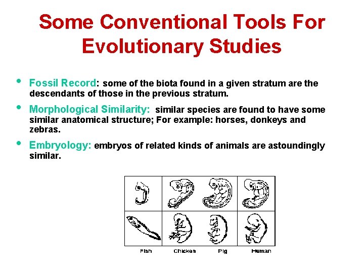
Some Conventional Tools For Evolutionary Studies • Fossil Record: some of the biota found in a given stratum are the • Morphological Similarity: similar species are found to have some • descendants of those in the previous stratum. similar anatomical structure; For example: horses, donkeys and zebras. Embryology: embryos of related kinds of animals are astoundingly similar.

Evolutionary Studies • Early approaches – Based on anatomical features – Subjective derivation of evolutionary relationships • Some of them were later proved incorrect • Modern approaches – Based on DNA – Objective derivation of evolutionary relationships

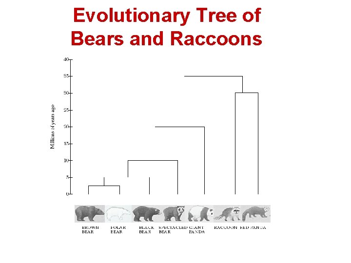
Success Story 1: the Giant Panda Riddle • • • For roughly 100 years scientists were unable to figure out which family the giant panda belongs to Giant pandas look like bears but have features that are unusual for bears and typical for raccoons, e. g. , they do not hibernate In 1985, Steven O’Brien and colleagues solved the giant panda classification problem using DNA sequences and algorithms

Evolutionary Tree of Bears and Raccoons

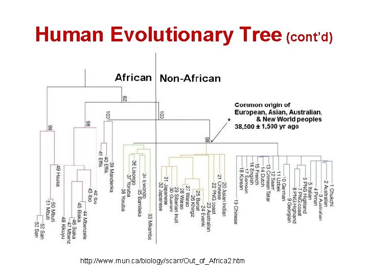
Success Story 2: Out of Africa Hypothesis • Around the time the giant panda riddle was solved, a DNA-based reconstruction of the human evolutionary tree lead to the Out of Africa Hypothesis: – Claims our most ancient ancestor lived in Africa roughly 200, 000 years ago

Human Evolutionary Tree (cont’d) http: //www. mun. ca/biology/scarr/Out_of_Africa 2. htm

How to construct such a tree?

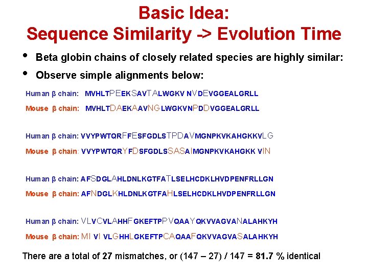
Basic Idea: Sequence Similarity -> Evolution Time • Beta globin chains of closely related species are highly similar: • Observe simple alignments below: Human β chain: MVHLTPEEKSAVTALWGKV NVDEVGGEALGRLL Mouse β chain: MVHLTDAEKAAVNGLWGKVNPDDVGGEALGRLL Human β chain: VVYPWTQRFFESFGDLSTPDAVMGNPKVKAHGKKVLG Mouse β chain: VVYPWTQRYFDSFGDLSSASAIMGNPKVKAHGKK VIN Human β chain: AFSDGLAHLDNLKGTFATLSELHCDKLHVDPENFRLLGN Mouse β chain: AFNDGLKHLDNLKGTFAHLSELHCDKLHVDPENFRLLGN Human β chain: VLVCVLAHHFGKEFTPPVQAAYQKVVAGVANALAHKYH Mouse β chain: MI VI VLGHHLGKEFTPCAQAAFQKVVAGVASALAHKYH There a total of 27 mismatches, or (147 – 27) / 147 = 81. 7 % identical

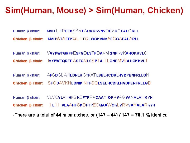
Sim(Human, Mouse) > Sim(Human, Chicken) Human β chain: MVH L TPEEKSAVTALWGKVNVDEVGGEALGRLL Chicken β chain: MVHWTAEEKQL Human β chain: VVYPWTQRFFESFGDLSTPDAVMGNPKVKAHGKKVLG Chicken β chain: IVYPWTQRFF ASFGNLSSPTA I LGNPMVRAHGKKVLT Human β chain: AFSDGLAHLDNLKGTFATLSELHCDKLHVDPENFRLLGN Chicken β chain: SFGDAVKNLDNIK NTFSQLSELHCDKLHVDPENFRLLGD Human β chain: VLVCVLAHHFGKEFTPPVQAAY QKVVAGVANALAHKYH Chicken β chain: I TGLWGKVNVAECGAEALARLL I I VLAAHFSKDFTPECQAAWQKLVRVVAHALARKYH -There a total of 44 mismatches, or (147 – 44) / 147 = 70. 1 % identical

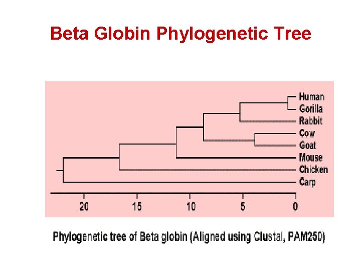
Beta Globin Phylogenetic Tree

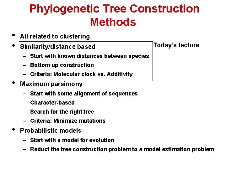
Phylogenetic Tree Construction Methods • • All related to clustering Similarity/distance based Today’s lecture – Start with known distances between species – Bottom up construction • – Criteria: Molecular clock vs. Additivity Maximum parsimony – Start with some alignment of sequences – Character-based – Search for the right tree • – Criteria: Minimize mutations Probabilistic models – Start with a model for evolution – Reduct the tree construction problem to a model estimation problem

Evolutionary Trees • • • Leaves represent existing species Internal vertices represent ancestors Rooted trees: – Root represents the oldest evolutionary ancestor – Can be viewed as directed trees from the root to the leaves • Unrooted trees: – The position of the root (“oldest ancestor”) is unknown. – Otherwise, they are like rooted trees

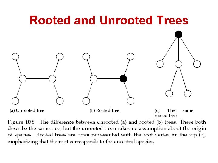
Rooted and Unrooted Trees

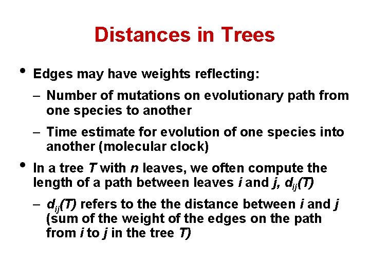
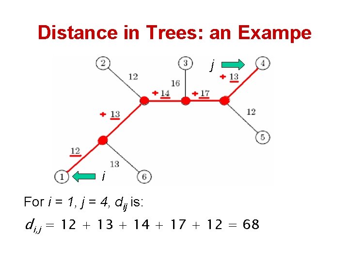
Distances in Trees • Edges may have weights reflecting: – Number of mutations on evolutionary path from one species to another – Time estimate for evolution of one species into another (molecular clock) • In a tree T with n leaves, we often compute the length of a path between leaves i and j, dij(T) – dij(T) refers to the distance between i and j (sum of the weight of the edges on the path from i to j in the tree T)

Distance in Trees: an Exampe j i For i = 1, j = 4, dij is: di, j = 12 + 13 + 14 + 17 + 12 = 68

Distance Matrix • Given n species, we can compute the n x n distance matrix Dij • Dij may be defined as the edit distance between a gene in species i and species j, where the gene of interest is sequenced for all n species. • Evolution of these genes is described by a tree that we don’t know. • We need an algorithm to construct a tree that best fits the distance matrix Dij

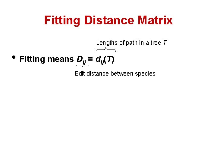
Fitting Distance Matrix Lengths of path in a tree T • Fitting means Dij = dij(T) Edit distance between species

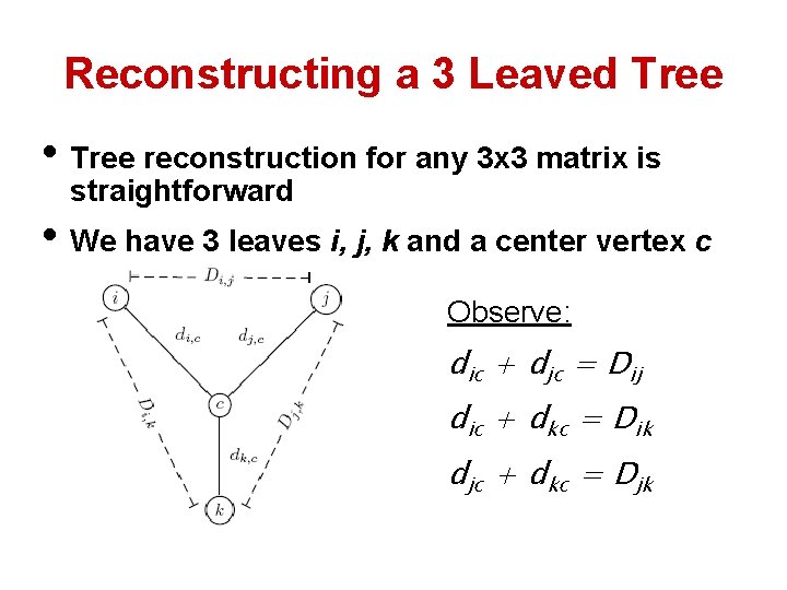
Reconstructing a 3 Leaved Tree • Tree reconstruction for any 3 x 3 matrix is straightforward • We have 3 leaves i, j, k and a center vertex c Observe: dic + djc = Dij dic + dkc = Dik djc + dkc = Djk

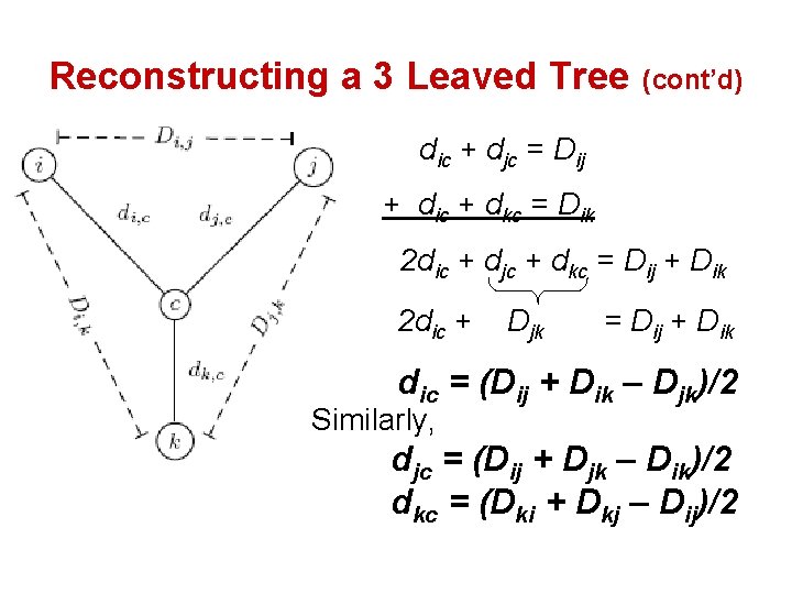
Reconstructing a 3 Leaved Tree (cont’d) dic + djc = Dij + dic + dkc = Dik 2 dic + djc + dkc = Dij + Dik 2 dic + Djk = Dij + Dik dic = (Dij + Dik – Djk)/2 Similarly, djc = (Dij + Djk – Dik)/2 dkc = (Dki + Dkj – Dij)/2

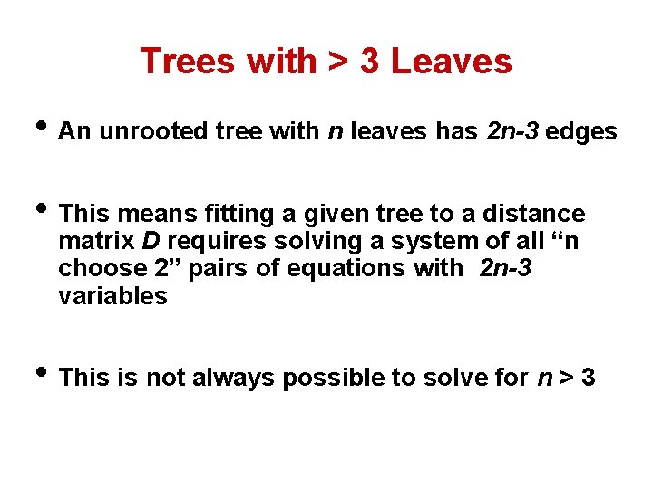
Trees with > 3 Leaves • An unrooted tree with n leaves has 2 n-3 edges • This means fitting a given tree to a distance matrix D requires solving a system of all “n choose 2” pairs of equations with 2 n-3 variables • This is not always possible to solve for n > 3

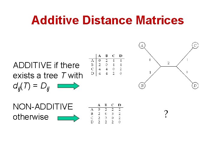
Additive Distance Matrices ADDITIVE if there exists a tree T with dij(T) = Dij NON-ADDITIVE otherwise

How do we know if a distance matrix is additive?

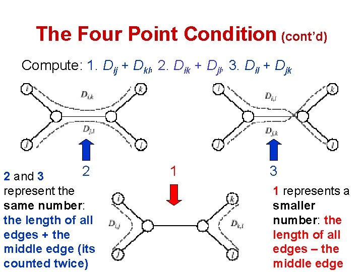
The Four Point Condition (cont’d) Compute: 1. Dij + Dkl, 2. Dik + Djl, 3. Dil + Djk 2 2 and 3 represent the same number: the length of all edges + the middle edge (its counted twice) 1 3 1 represents a smaller number: the length of all edges – the middle edge

The Four Point Condition: Theorem • The four point condition is satisfied if 2 of these sums are the same number, with the third sum smaller than these first two • Theorem : An n x n matrix D is additive if and only if the four point condition holds for every 4 distinct elements 1 ≤ i, j, k, l ≤ n

Distance Based Phylogeny Problem • Goal: Reconstruct an evolutionary tree from a distance matrix • Input: n x n distance matrix Dij • Output: weighted unrooted tree T with n leaves fitting D • If D is additive, this problem has a solution and there is a simple algorithm to solve it

Neighboring Leaves • Find neighboring leaves i and j with parent k • Remove the rows and columns of i and j • Add a new row and column corresponding to k, where the distance from k to any other leaf m can be computed by: Dkm = (Dim + Djm – Dij)/2 Compress i and j into k, iterate algorithm for rest of tree

Finding Neighboring Leaves • To find neighboring leaves we simply select a pair of closest leaves.

Finding Neighboring Leaves • To find neighboring leaves we simply select a pair of closest leaves. WRONG

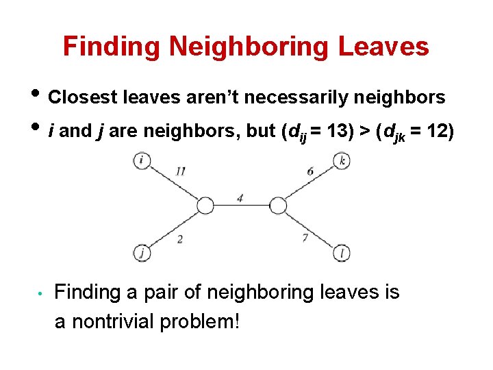
Finding Neighboring Leaves • Closest leaves aren’t necessarily neighbors • i and j are neighbors, but (dij = 13) > (djk = 12) • Finding a pair of neighboring leaves is a nontrivial problem!

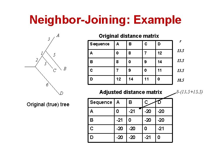
Neighbor Joining Algorithm • • • In 1987 Naruya Saitou and Masatoshi Nei developed a neighbor joining algorithm for phylogenetic tree reconstruction Finds a pair of leaves that are close to each other but far from other leaves: implicitly finds a pair of neighboring leaves Advantages: works for both additive and non-additive matrices

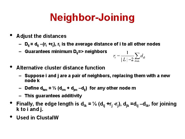
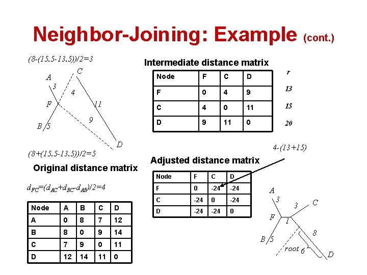
Neighbor-Joining • Adjust the distances – Dij = dij –(ri +rj), ri is the average distance of i to all other nodes – Guarantees minimum Dij=> neighbors • Alternative cluster distance function – Suppose i and j are a pair of neighbors, replacing them with a new node k – Define dkm = ½ (dim + djm –dij) for any other node m • • – This guarantees additivity Finally, the edge length is dik = ½ (dij +rj -rj), djk =dij –dik, for joining k to i and j. Used in Clustal. W

Neighbor-Joining: Example A 3 1 2 Original distance matrix 5 3 B C A B C D A 0 8 7 12 B 8 0 9 14 15. 5 C 7 9 0 11 13. 5 D 12 14 11 0 18. 5 6 Adjusted distance matrix D Original (true) tree r Sequence A B C D A 0 -21 -20 B -21 0 -20 C -20 0 -21 D -20 -21 0 13. 5 8 -(13. 5+15. 5)

Neighbor-Joining: Example (cont. ) (8 -(15. 5 -13. 5))/2=3 Intermediate distance matrix C A 3 4 F 11 9 B 5 F C D F 0 4 9 13 C 4 0 11 15 D 9 11 0 20 D (8+(15. 5 -13. 5))/2=5 Original distance matrix d. FC=(d. AC+d. BC-d. AB)/2=4 Node A B C D A 0 8 7 12 B 8 0 9 14 C 7 9 0 11 D 12 14 11 0 r Node 4 -(13+15) Adjusted distance matrix Node F C D F 0 -24 C -24 0 -24 D -24 0 A 3 F 3 C 1 8 B 5 root 6 D

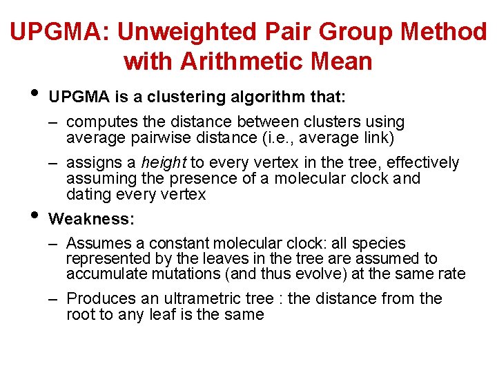
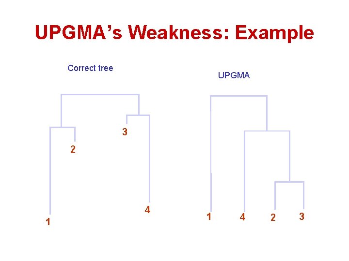
UPGMA: Unweighted Pair Group Method with Arithmetic Mean • • UPGMA is a clustering algorithm that: – computes the distance between clusters using average pairwise distance (i. e. , average link) – assigns a height to every vertex in the tree, effectively assuming the presence of a molecular clock and dating every vertex Weakness: – Assumes a constant molecular clock: all species represented by the leaves in the tree are assumed to accumulate mutations (and thus evolve) at the same rate – Produces an ultrametric tree : the distance from the root to any leaf is the same

UPGMA’s Weakness: Example Correct tree UPGMA 3 2 4 1 1 4 2 3

Least Squares Distance Phylogeny Problem • If the distance matrix D is NOT additive, then we look for a tree T that approximates D the best: Squared Error : ∑i, j (dij(T) – Dij)2 • • Squared Error is a measure of the quality of the fit between distance matrix and the tree: we want to minimize it. Least Squares Distance Phylogeny Problem: finding the best approximation tree T for a non-additive matrix D (NP-hard).

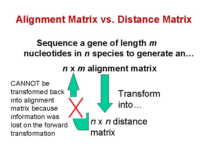
Alignment Matrix vs. Distance Matrix Sequence a gene of length m nucleotides in n species to generate an… n x m alignment matrix CANNOT be transformed back into alignment matrix because information was lost on the forward transformation Transform into… n x n distance matrix

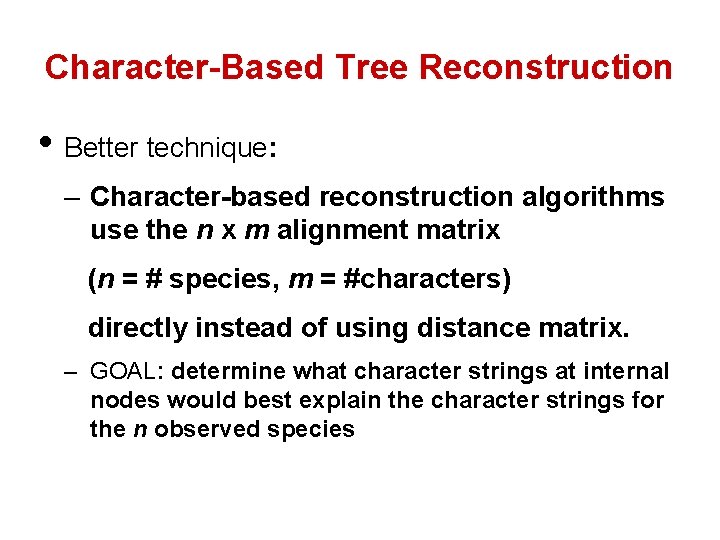
Character-Based Tree Reconstruction • Better technique: – Character-based reconstruction algorithms use the n x m alignment matrix (n = # species, m = #characters) directly instead of using distance matrix. – GOAL: determine what character strings at internal nodes would best explain the character strings for the n observed species

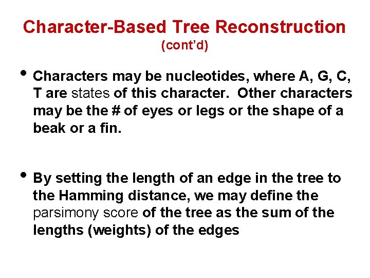
Character-Based Tree Reconstruction (cont’d) • Characters may be nucleotides, where A, G, C, T are states of this character. Other characters may be the # of eyes or legs or the shape of a beak or a fin. • By setting the length of an edge in the tree to the Hamming distance, we may define the parsimony score of the tree as the sum of the lengths (weights) of the edges

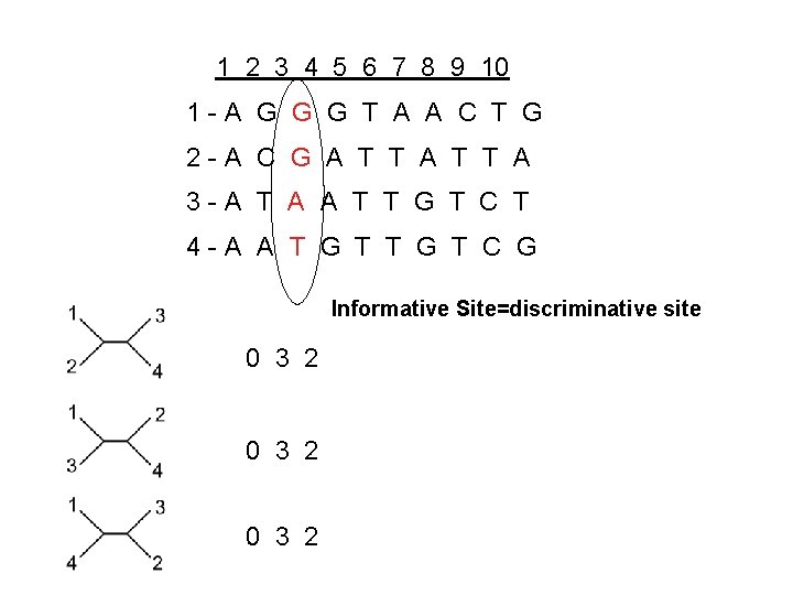
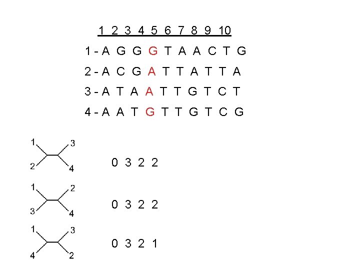
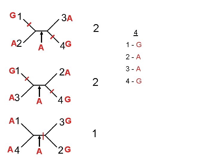
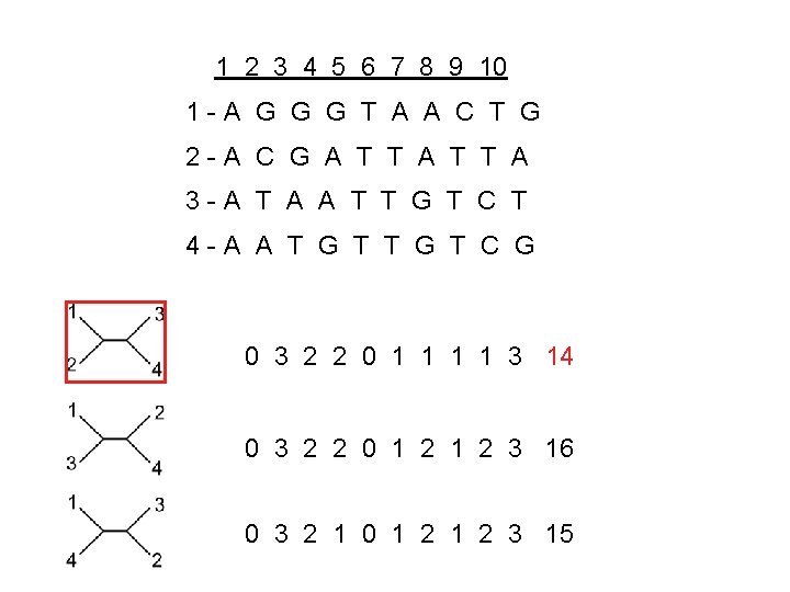
Maximum Parsimony maximum parsimony principle: the principle that the most accurate phylogenetic tree is one that is based on the fewest changes in the genetic code.

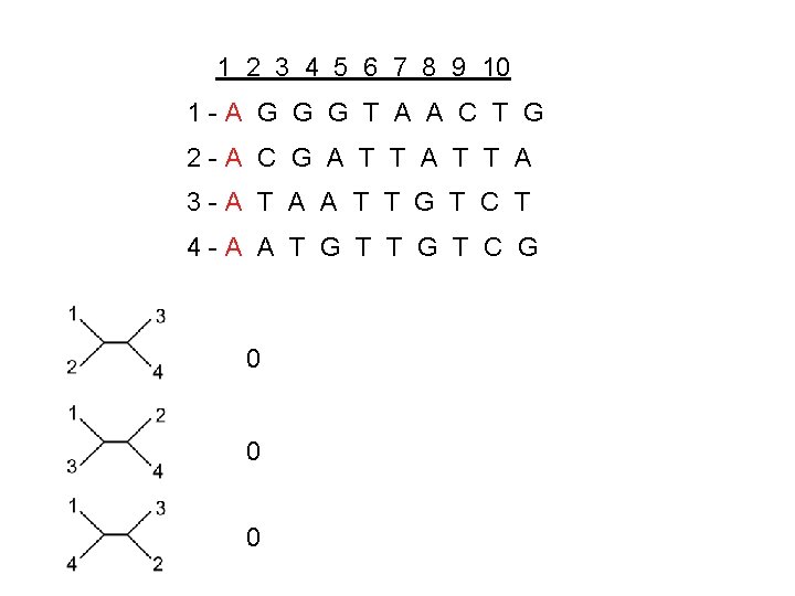
1 2 3 4 5 6 7 8 9 10 1 -A G G G T A A C T G 2 -A C G A T T A 3 -A T A A T T G T C T 4 -A A T G T C G 0 0 0

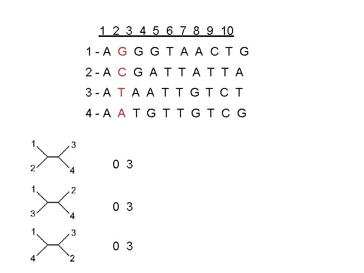
1 2 3 4 5 6 7 8 9 10 1 -A G G G T A A C T G 2 -A C G A T T A 3 -A T A A T T G T C T 4 -A A T G T C G 0 3 0 3

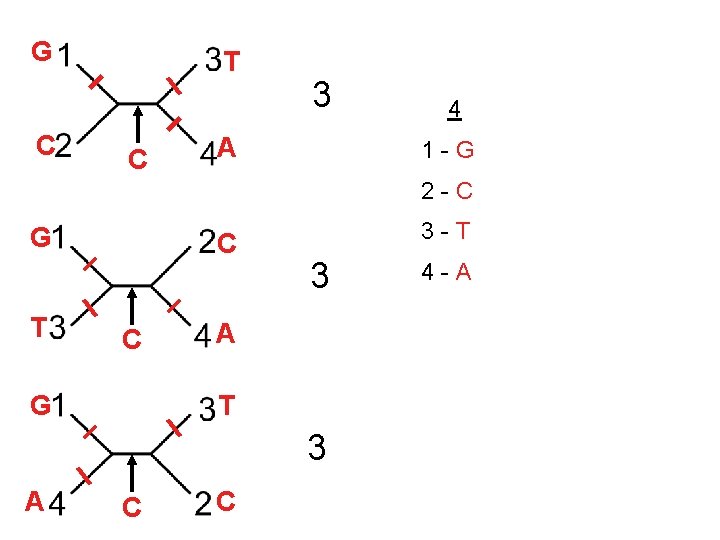
G C T C 3 A 4 1 -G 2 -C G T C C G 3 -T 3 A C C 4 -A

1 2 3 4 5 6 7 8 9 10 1 -A G G G T A A C T G 2 -A C G A T T A 3 -A T A A T T G T C T 4 -A A T G T C G Informative Site=discriminative site 0 3 2

1 2 3 4 5 6 7 8 9 10 1 -A G G G T A A C T G 2 -A C G A T T A 3 -A T A A T T G T C T 4 -A A T G T C G 0 3 2 2 0 3 2 1

G A A A 2 G 4 1 -G 2 -A G A A 3 -A 2 G G 1 A A G 4 -G

1 2 3 4 5 6 7 8 9 10 1 -A G G G T A A C T G 2 -A C G A T T A 3 -A T A A T T G T C T 4 -A A T G T C G 0 3 2 2 0 3 2 1

1 2 3 4 5 6 7 8 9 10 1 -A G G G T A A C T G 2 -A C G A T T A 3 -A T A A T T G T C T 4 -A A T G T C G 0 3 2 2 0 1 1 3 14 0 3 2 2 0 1 2 3 16 0 3 2 1 0 1 2 3 15

Small Parsimony Problem • Input: Tree T with each leaf labeled by an mcharacter string. • Output: Labeling of internal vertices of the tree T minimizing the parsimony score. • We can assume that every leaf is labeled by a single character, because the characters in the string are independent.

Weighted Small Parsimony Problem • A more general version of Small Parsimony Problem • Input includes a k * k scoring matrix describing the cost of transformation of each of k states into another one

Sankoff’s Algorithm • Build from leaves to the root • Then move down and assign each node with its character. • The character at each leave and internal vertex isn’t determined until the root is determined. • Need to keep tract of every character.

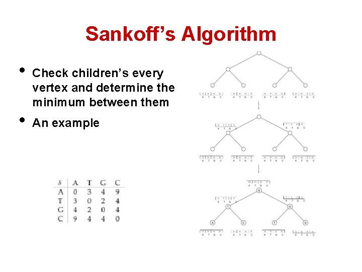
Sankoff’s Algorithm • • Check children’s every vertex and determine the minimum between them An example

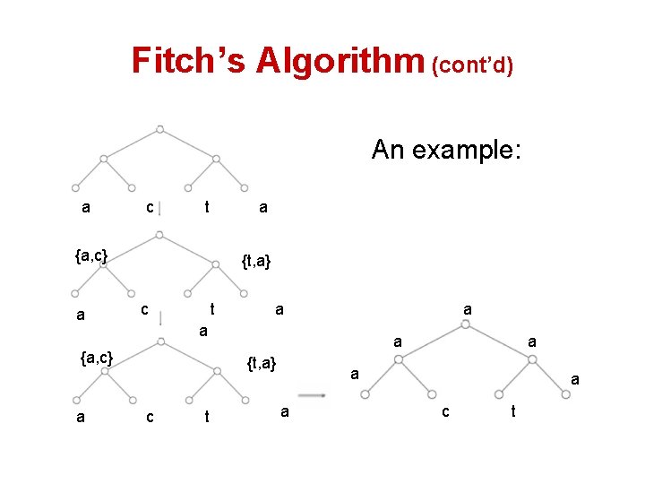
Fitch’s Algorithm • Solves Small Parsimony problem • Dynamic programming in essence • Assigns a set of letter to every vertex in the tree. • If the two children’s sets of character overlap, it’s the common set of them • If not, it’s the combined set of them.

Fitch’s Algorithm (cont’d) An example: a c t a {a, c} a {t, a} c t a a {a, c} a a a {t, a} c t a a c t

Probabilistic Approaches • Basic idea: – Tree= Generative probabilistic model, e. g. , an n-leaf tree defines a model p(X 1, …, Xn) – Data: sequences {s 1, …, sn} – Choose the tree according to • Maximum Likelihood: p(Data|Tree) • Maximum A Posterior (Bayesian): p(Tree|Data) • Model evolution more directly • Computationally expensive

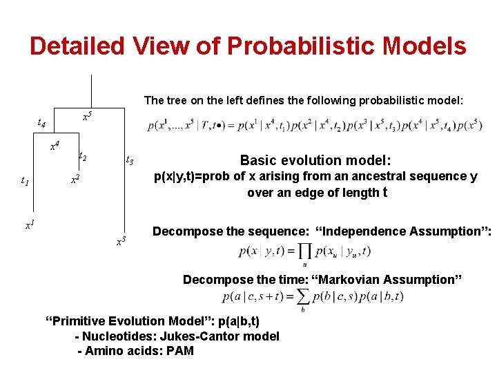
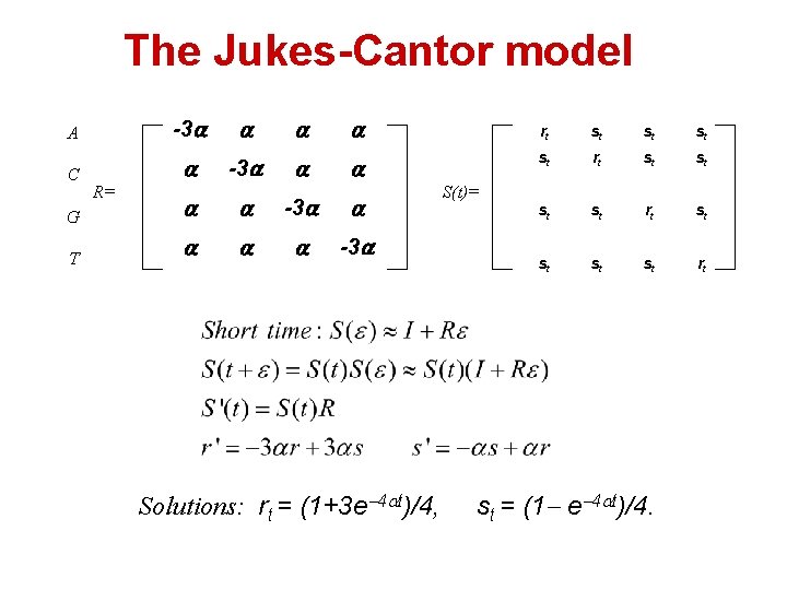
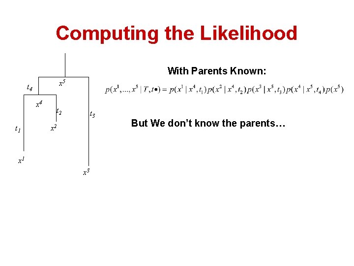
Detailed View of Probabilistic Models The tree on the left defines the following probabilistic model: x 5 t 4 x 4 t 1 t 2 t 3 Basic evolution model: p(x|y, t)=prob of x arising from an ancestral sequence y over an edge of length t x 2 x 1 x 3 Decompose the sequence: “Independence Assumption”: Decompose the time: “Markovian Assumption” “Primitive Evolution Model”: p(a|b, t) - Nucleotides: Jukes-Cantor model - Amino acids: PAM

The Jukes-Cantor model A -3 C -3 R= G -3 T -3 Solutions: rt = (1+3 e 4 t)/4, rt st st rt st st rt S(t)= st = (1 e 4 t)/4.

Computing the Likelihood With Parents Known: x 5 t 4 x 4 t 1 t 2 t 3 x 2 x 1 x 3 But We don’t know the parents…

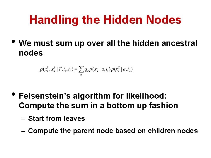
Handling the Hidden Nodes • We must sum up over all the hidden ancestral nodes • Felsenstein’s algorithm for likelihood: Compute the sum in a bottom up fashion – Start from leaves – Compute the parent node based on children nodes

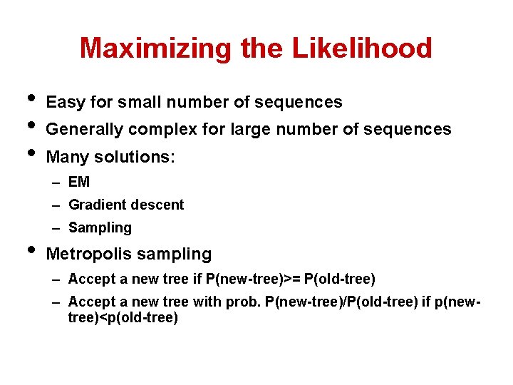
Maximizing the Likelihood • • • Easy for small number of sequences Generally complex for large number of sequences Many solutions: – EM – Gradient descent • – Sampling Metropolis sampling – Accept a new tree if P(new-tree)>= P(old-tree) – Accept a new tree with prob. P(new-tree)/P(old-tree) if p(newtree)<p(old-tree)

More realistic evolutionary models • Allowing different rates at different sites – Using a prior (e. g. , gamma) to regular the different rates – Hidden Markov models • Evolutionary models with gaps – Tree HMMs

What You Should Know • What is a phylogenetic tree (rooted, unrooted) • How the neighbor-joining algorithm works • Know the basic idea of maximum parsimony