Essential CS Statistics Lecture for CS 498 CXZ

Essential CS & Statistics (Lecture for CS 498 -CXZ Algorithms in Bioinformatics) Aug. 30, 2005 Cheng. Xiang Zhai Department of Computer Science University of Illinois, Urbana-Champaign

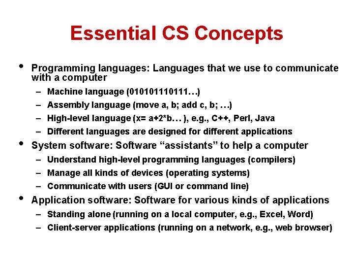
Essential CS Concepts • • • Programming languages: Languages that we use to communicate with a computer – – Machine language (01010111…) Assembly language (move a, b; add c, b; …) High-level language (x= a+2*b… ), e. g. , C++, Perl, Java Different languages are designed for different applications System software: Software “assistants” to help a computer – Understand high-level programming languages (compilers) – Manage all kinds of devices (operating systems) – Communicate with users (GUI or command line) Application software: Software for various kinds of applications – Standing alone (running on a local computer, e. g. , Excel, Word) – Client-server applications (running on a network, e. g. , web browser)

Intelligence/Capacity of a Computer • The intelligence of a computer is determined • by the intelligence of the software it can run Capacities of a computer for running software mainly determined by its – Speed – Memory – Disk space • Given a particular computer, we would like to write software that is highly intelligent, that can run fast, and that doesn’t need much memory (contradictory goals)

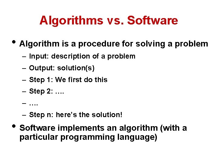
Algorithms vs. Software • Algorithm is a procedure for solving a problem – Input: description of a problem – Output: solution(s) – Step 1: We first do this – Step 2: …. – Step n: here’s the solution! • Software implements an algorithm (with a particular programming language)

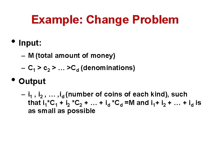
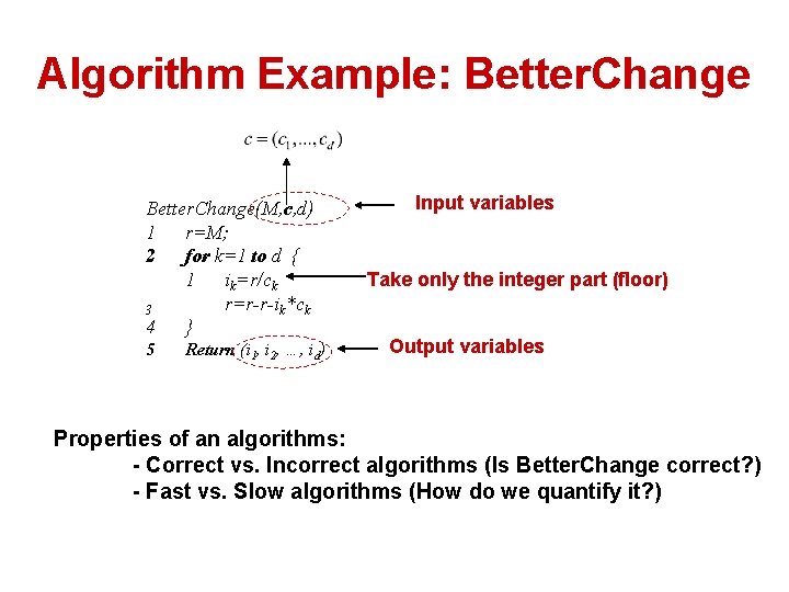
Example: Change Problem • Input: – M (total amount of money) – C 1 > c 2 > … >Cd (denominations) • Output – i 1 , i 2 , … , id (number of coins of each kind), such that i 1*C 1 + i 2 *C 2 + … + id *Cd =M and i 1+ i 2 + … + id is as small as possible

Algorithm Example: Better. Change(M, c, d) 1 r=M; 2 for k=1 to d { 1 ik=r/ck r=r-r-ik*ck 3 4 } 5 Return (i 1, i 2, …, id) Input variables Take only the integer part (floor) Output variables Properties of an algorithms: - Correct vs. Incorrect algorithms (Is Better. Change correct? ) - Fast vs. Slow algorithms (How do we quantify it? )

Big-O Notation • How can we compare the running time of two algorithms in a computer-independent way? • Observations: – In general, as the problem size grows, the running time increases (sorting 500 numbers would take more time than sorting 5 elements) – Running time is more critical for large problem size (think about sorting 5 numbers vs. sorting 50000 numbers) • How about measuring the growth rate of running time?

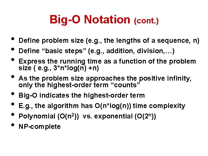
Big-O Notation (cont. ) • • Define problem size (e. g. , the lengths of a sequence, n) Define “basic steps” (e. g. , addition, division, …) Express the running time as a function of the problem size ( e. g. , 3*n*log(n) +n) As the problem size approaches the positive infinity, only the highest-order term “counts” Big-O indicates the highest-order term E. g. , the algorithm has O(n*log(n)) time complexity Polynomial (O(n 2)) vs. exponential (O(2 n)) NP-complete

Basic Probability & Statistics

Purpose of Prob. & Statistics • Deductive vs. Plausible reasoning • Incomplete knowledge -> uncertainty • How do we quantify inference under uncertainty? – Probability: models of random process/experiments (how data are generated) – Statistics: draw conclusions on the whole population based on samples (inference on data)

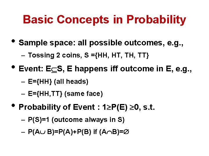
Basic Concepts in Probability • Sample space: all possible outcomes, e. g. , – Tossing 2 coins, S ={HH, HT, TH, TT} • Event: E S, E happens iff outcome in E, e. g. , – E={HH} (all heads) – E={HH, TT} (same face) • Probability of Event : 1 P(E) 0, s. t. – P(S)=1 (outcome always in S) – P(A B)=P(A)+P(B) if (A B)=

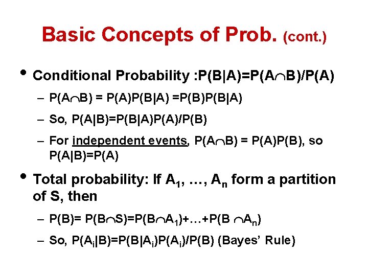
Basic Concepts of Prob. (cont. ) • Conditional Probability : P(B|A)=P(A B)/P(A) – P(A B) = P(A)P(B|A) =P(B)P(B|A) – So, P(A|B)=P(B|A)P(A)/P(B) – For independent events, P(A B) = P(A)P(B), so P(A|B)=P(A) • Total probability: If A 1, …, An form a partition of S, then – P(B)= P(B S)=P(B A 1)+…+P(B An) – So, P(Ai|B)=P(B|Ai)P(Ai)/P(B) (Bayes’ Rule)

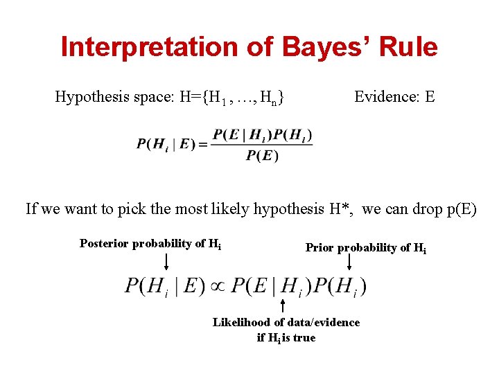
Interpretation of Bayes’ Rule Hypothesis space: H={H 1 , …, Hn} Evidence: E If we want to pick the most likely hypothesis H*, we can drop p(E) Posterior probability of Hi Prior probability of Hi Likelihood of data/evidence if Hi is true

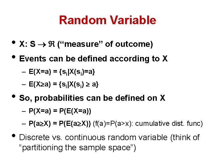
Random Variable • X: S (“measure” of outcome) • Events can be defined according to X – E(X=a) = {si|X(si)=a} – E(X a) = {si|X(si) a} • So, probabilities can be defined on X – P(X=a) = P(E(X=a)) – P(a X) = P(E(a X)) (f(a)=P(a>x): cumulative dist. func) • Discrete vs. continuous random variable (think of “partitioning the sample space”)

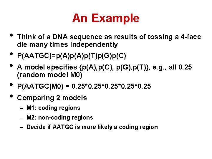
An Example • • • Think of a DNA sequence as results of tossing a 4 -face die many times independently P(AATGC)=p(A)p(T)p(G)p(C) A model specifies {p(A), p(C), p(G), p(T)}, e. g. , all 0. 25 (random model M 0) P(AATGC|M 0) = 0. 25*0. 25 Comparing 2 models – M 1: coding regions – M 2: non-coding regions – Decide if AATGC is more likely a coding region

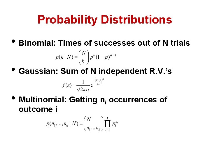
Probability Distributions • Binomial: Times of successes out of N trials • Gaussian: Sum of N independent R. V. ’s • Multinomial: Getting ni occurrences of outcome i

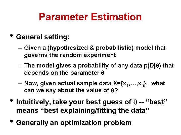
Parameter Estimation • General setting: – Given a (hypothesized & probabilistic) model that governs the random experiment – The model gives a probability of any data p(D| ) that depends on the parameter – Now, given actual sample data X={x 1, …, xn}, what can we say about the value of ? • Intuitively, take your best guess of -- “best” means “best explaining/fitting the data” • Generally an optimization problem

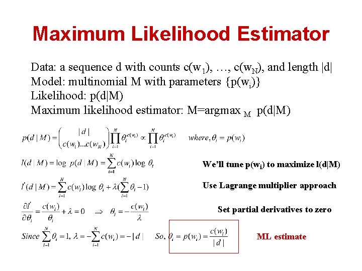
Maximum Likelihood Estimator Data: a sequence d with counts c(w 1), …, c(w. N), and length |d| Model: multinomial M with parameters {p(wi)} Likelihood: p(d|M) Maximum likelihood estimator: M=argmax M p(d|M) We’ll tune p(wi) to maximize l(d|M) Use Lagrange multiplier approach Set partial derivatives to zero ML estimate

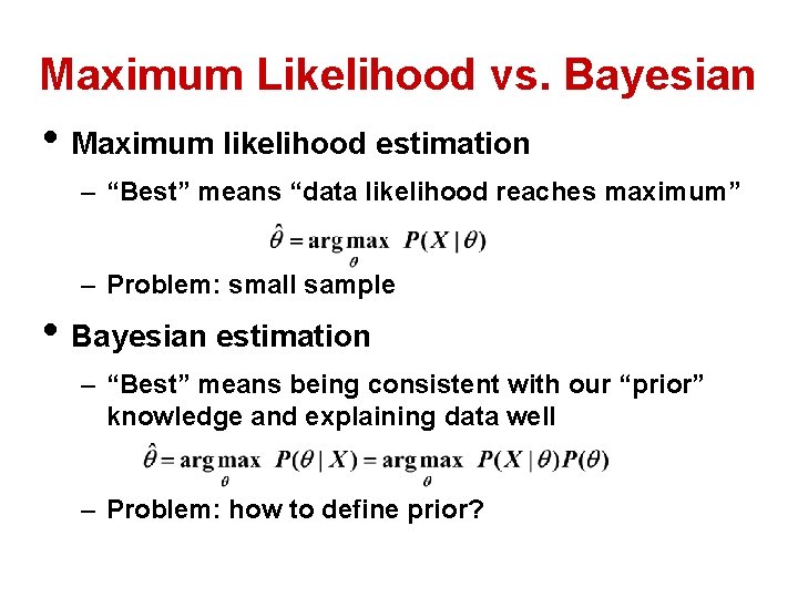
Maximum Likelihood vs. Bayesian • Maximum likelihood estimation – “Best” means “data likelihood reaches maximum” – Problem: small sample • Bayesian estimation – “Best” means being consistent with our “prior” knowledge and explaining data well – Problem: how to define prior?

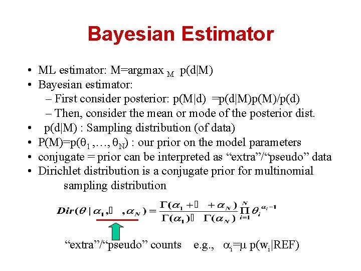
Bayesian Estimator • ML estimator: M=argmax M p(d|M) • Bayesian estimator: – First consider posterior: p(M|d) =p(d|M)p(M)/p(d) – Then, consider the mean or mode of the posterior dist. • p(d|M) : Sampling distribution (of data) • P(M)=p( 1 , …, N) : our prior on the model parameters • conjugate = prior can be interpreted as “extra”/“pseudo” data • Dirichlet distribution is a conjugate prior for multinomial sampling distribution “extra”/“pseudo” counts e. g. , i= p(wi|REF)

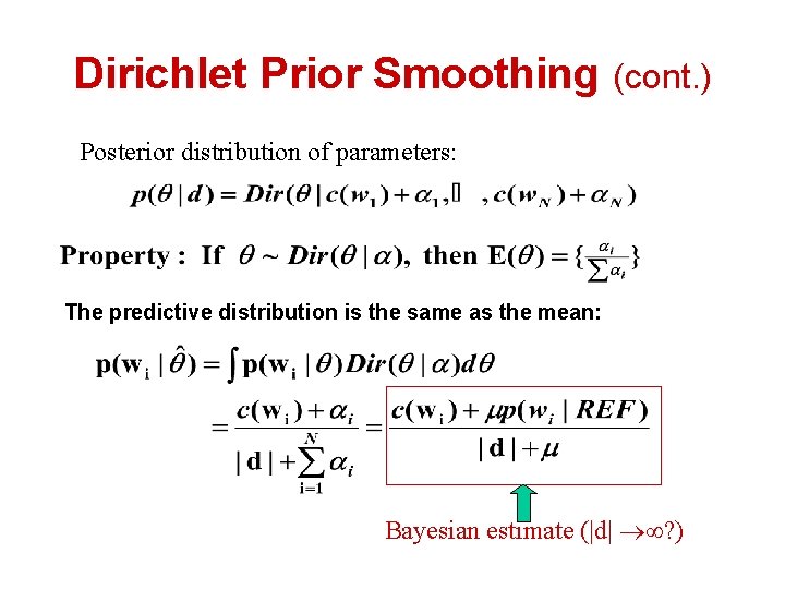
Dirichlet Prior Smoothing (cont. ) Posterior distribution of parameters: The predictive distribution is the same as the mean: Bayesian estimate (|d| ? )

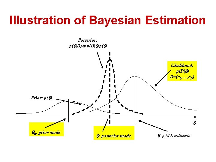
Illustration of Bayesian Estimation Posterior: p( |D) p(D| )p( ) Likelihood: p(D| ) D=(c 1, …, c. N) Prior: p( ) : prior mode : posterior mode ml: ML estimate

Basic Concepts in Information Theory • Entropy: Measuring uncertainty of a random variable • Kullback-Leibler divergence: comparing two distributions • Mutual Information: measuring the correlation of two random variables

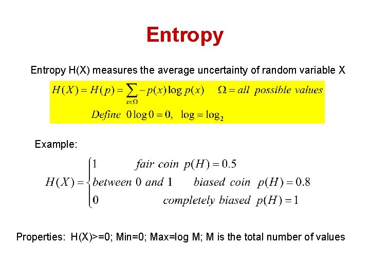
Entropy H(X) measures the average uncertainty of random variable X Example: Properties: H(X)>=0; Min=0; Max=log M; M is the total number of values

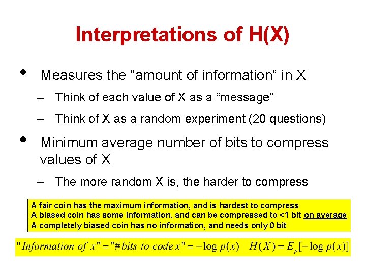
Interpretations of H(X) • Measures the “amount of information” in X – Think of each value of X as a “message” – Think of X as a random experiment (20 questions) • Minimum average number of bits to compress values of X – The more random X is, the harder to compress A fair coin has the maximum information, and is hardest to compress A biased coin has some information, and can be compressed to <1 bit on average A completely biased coin has no information, and needs only 0 bit

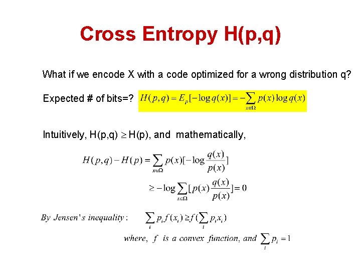
Cross Entropy H(p, q) What if we encode X with a code optimized for a wrong distribution q? Expected # of bits=? Intuitively, H(p, q) H(p), and mathematically,

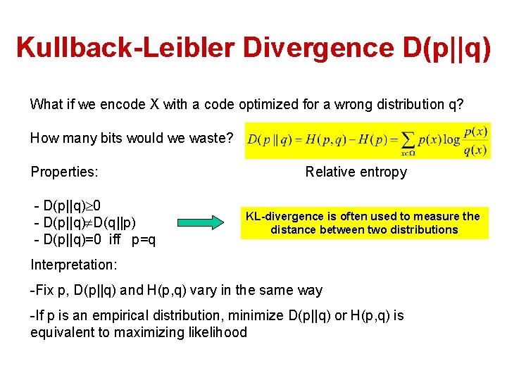
Kullback-Leibler Divergence D(p||q) What if we encode X with a code optimized for a wrong distribution q? How many bits would we waste? Properties: - D(p||q) 0 - D(p||q) D(q||p) - D(p||q)=0 iff p=q Relative entropy KL-divergence is often used to measure the distance between two distributions Interpretation: -Fix p, D(p||q) and H(p, q) vary in the same way -If p is an empirical distribution, minimize D(p||q) or H(p, q) is equivalent to maximizing likelihood

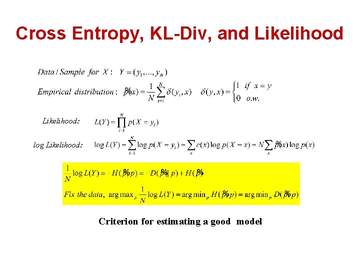
Cross Entropy, KL-Div, and Likelihood: log Likelihood: Criterion for estimating a good model

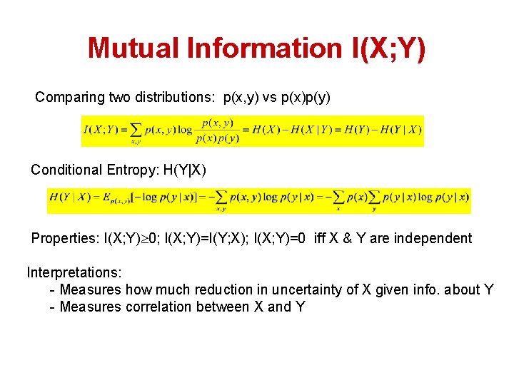
Mutual Information I(X; Y) Comparing two distributions: p(x, y) vs p(x)p(y) Conditional Entropy: H(Y|X) Properties: I(X; Y) 0; I(X; Y)=I(Y; X); I(X; Y)=0 iff X & Y are independent Interpretations: - Measures how much reduction in uncertainty of X given info. about Y - Measures correlation between X and Y

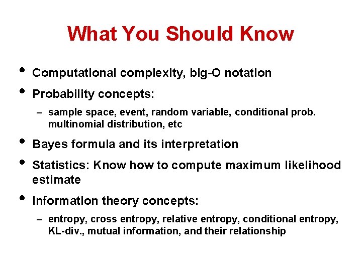
What You Should Know • • Computational complexity, big-O notation Probability concepts: – sample space, event, random variable, conditional prob. multinomial distribution, etc • • • Bayes formula and its interpretation Statistics: Know how to compute maximum likelihood estimate Information theory concepts: – entropy, cross entropy, relative entropy, conditional entropy, KL-div. , mutual information, and their relationship