FIN 30210 Managerial Economics Cost Analysis Heres the

FIN 30210: Managerial Economics Cost Analysis

Here’s the overall objective for the firm Factor Markets Businesses take factor prices as given Production Decisions Factor Usage/Prices Determine Production Costs You are here Product Markets Demand market structure determine the markup of price over cost Coming Soon

Example: Moneyball - The Art of Winning an Unfair Game Michael Lewis

What is Billy Beane’s Problem…No Money! Final Standings W/L: 103/58 WP: . 640 Dollars/Win: $1. 36 M Final Standings W/L: 103/59 WP: . 636 Dollars/Win: $388 K As a small market team, the A’s were pretty near the bottom in terms of payrolls, but they made every dollar count! 2002 Major League Payrolls

What is Billy Beane’s Objective? Minimize costs for a given production level (potentially subject to one or more constraints) Billy Beane is looking for the cheapest way for the Oakland A’s to win the world series OR Maximize production levels while operating within a given budget Billy Beane and would like to maximize the production of the Oakland A’s while staying within payroll limits.

Enter Paul De. Podesta (a. k. a. Peter Brand) Can we define a Production Function for a Baseball Club? Billy Beane Paul De. Podesta Output = Wins Brad Pitt as Billy Beane Jonah Hill as “Peter Brand” Inputs = Players Winning Percentage RS = Runs Scored RA = Runs Given up Bill James

Winning Percentage For a team with the league average runs against, here’s what this looks like 1 In 2015, the league average was 688 0, 9 0, 8 0, 7 0, 6 0, 5 0, 4 0, 3 0, 2 0, 1 0 0 200 400 600 800 1000 1200 1400 1600 1800 2000 Runs Scored

For a fixed number of runs against, hitting homers does have diminishing returns! 1 0, 001 League Range tage n e c r 0, 9 0, 0009 e g. P n in W 0, 0008 0, 7 0, 0007 0, 6 0, 0006 0, 5 0, 0005 0, 4 0, 0004 0, 3 0, 0003 Cha nge 0, 2 Change Winning Percentage 0, 8 In 2015, the league average was 688 0, 0002 0, 1 0, 0001 0 0 0 200 400 600 800 1000 1200 1400 1600 1800 2000 Runs Scored

For a fixed number of runs for, runs against also has diminishing returns! 1, 2 0, 001 League Range 0, 0009 1 0, 0008 0, 0007 0, 8 ge n a 0, 6 0, 4 0, 0006 Ch 0, 0005 age t n e erc 0, 0004 Winn ing P 0, 0003 0, 0002 0, 0001 0 1000 0 800 600 400 200 Runs Against In 2015, the league average was 688

Let’s look at the Cubs vs. The Yankees Predicted Winning Percentage 1 League Range 0, 9 0, 8 0, 7 . 562. 545 0, 6 For the Yankees to match the Cubs win percentage, they would need 800 runs 0, 5 Chicago Cubs (2015) Total Payroll: $120, 337, 385 Avg. Salary: $3, 760, 543 Wins/Losses: 97/65 WP: . 598 RS: 689 RA: 608 Dollars/Win: $1, 240, 591 New York Yankees (2015) Total Payroll: $217, 758, 751 Avg. Salary: $7, 258, 619 Wins/Losses: 87/75 WP: . 537 RS: 764 RA: 698 Dollars/Win: $2, 502, 974 0, 3 0, 2 0, 1 0 0 200 400 600 800 1000 1200 1400 1600 1800 2000 2200 2400 2600 Runs Scored

To evaluate a player’s contribution to run production, numerous statistics are derived On Base Percentage H = Hits W = Walks HBP = Hit by Pitch AB = At Bats SF = Sacrifice Flies Runs Created H = Hits W = Walks TB = Total Bases AB = At Bats Peter Brand: “It's about getting things down to one number. Using the stats the way we read them, we'll find value in players that no one else can see”

So, let’s evaluate a couple possible players to help the Yankees catch up to the Cubs Runs Created H = Hits W = Walks TB = Total Bases AB = At Bats Albert Pujols (L. A. Angels) 2015 Salary: $25, 000 H = 147 W = 50 TB = 289 AB = 602 H = 147 W = 50 HBP = 6 AB = 602 SF = 3 On Base Percentage H = Hits W = Walks HBP = Hit by Pitch AB = At Bats SF = Sacrifice Flies Bryce Harper (Washington Nationals) 2015 Salary: $5, 000 H = 172 W = 124 TB = 338 AB = 521 H = 172 W = 124 HBP = 5 AB = 521 SF = 4

Winning Percentage With Bryce Harper 1 New York Yankees Total Payroll: $217, 758, 751 +$ 5, 000 $222, 758, 751 RS: 764 + 155 = 919 RA: 698 WP: . 634 League Range 0, 9 0, 8 0, 7 . 562. 545 0, 6 0, 5 With Albert Pujols 0, 4 0, 3 0, 2 0, 1 0 0 200 400 600 800 1000 1200 1400 1600 1800 2000 2200 2400 Runs Scored 2600 New York Yankees (2015) Total Payroll: $217, 758, 751 +$ 25, 000 $242, 758, 751 RS: 764 + 87 = 851 RA: 698 WP: . 597

Can we apply “Moneyball” more generally? Minimize costs for a given production level (potentially subject to one or more constraints) Example: PG&E would like to meet the daily electricity demands of its 5. 1 Million customers for the lowest possible cost Or Maximize production levels while operating within a given budget Example: Notre Dame wants to maximize it’s educational/research output given its budgetary limitations

You produce a single output. There is no distinction as far as quality is concerned, so all we are concerned with is quantity. You require two types of input in your production process (capital and labor). Labor inputs can be adjusted instantaneously, but capital adjustments require at least 1 year Total Production “Is a function of” Capital (Fixed for any planning horizon under 1 year Labor (always adjustable)

We have several performance metrics for inputs Marginal Product: marginal product measures the change in total production associated with a small change in one factor, holding all other factors fixed Average Product: average product measures the ratio of input to output Elasticity of Production: marginal product measures the change in total production associated with a small change in one factor, holding all other factors fixed

Over a short planning horizon, when many factors are considered fixed (in this case, capital), the key property of production is the marginal product of labor. Diminishing Marginal Returns: As labor input increases, production increases, but at a decreasing rate Increasing Marginal Returns: As labor input increases, production increases at an increasing rate

Note that the behavior of marginal product influences average product. Diminishing Marginal Returns: As labor input increases, the marginal product decreases and pulls the average down Increasing Marginal Returns: As labor input increases, marginal product increases and pulls the average up

Often, a production process will display both characteristics. Increasing Marginal Returns: As labor input increases, marginal product increases and pulls the average up Diminishing Marginal Returns: As labor input increases, the marginal product decreases and pulls the average down

Example: Baseball Winning Percentage 1 0, 001 tage n e c r 0, 9 0, 0009 e g. P n in W 0, 0008 0, 7 0, 0007 0, 6 0, 0006 0, 5 0, 0005 0, 4 0, 0004 0, 3 0, 0003 Cha nge 0, 2 Change Winning Percentage 0, 8 In 2015, the league average was 688 0, 0002 0, 1 0, 0001 0 0 0 200 400 600 800 1000 1200 1400 1600 Increasing Marginal Returns: As Diminishing Marginal Returns: As labor input increases, the labor input increases, marginal product decreases product increases 1800 2000 Runs Scored

Suppose we minimize total costs for a fixed capital stock This is a fixed cost in the short run So, minimizing the total costs associated with producing a set quantity of output would look like this NOTE: With the capital stock, this is a rather trivial problem. There is only one choice for labor that gets the job done. Bear with me…there is a reason for doing this!

Suppose we minimize total costs for a fixed capital stock First, write down the lagrangian…. We have one minimization condition and a constraint NOTE: With the capital stock fixed, this is a rather trivial problem. There is only one choice for labor that gets the job done. Bear with me…there is a reason for doing this! Recall that the multiplier measures the marginal impact of the constraint. In this case, it would be the impact on costs of altering the production level…marginal cost!

Now, imagine varying the quantity constraint Remember, lambda gives you marginal cost Every choice for quantity will have a choice for labor associated with it. Maximum Efficiency!! (Minimum Marginal Cost)

Alternatively, we could maximize production given a fixed budget Again, write down the lagrangian…. Again, we have one minimization condition and a constraint NOTE: With the capital stock fixed, this is a rather trivial problem. There is only one choice for labor that gets the job done. Bear with me…there is a reason for doing this! Recall that the multiplier measures the marginal impact of the constraint. In this case, it would be the impact on production of altering the budget!

Now, imagine varying the cost constraint Remember, lambda gives you output per dollar Every value for the cost constraint implies an affordable choice for labor Maximum Efficiency!! (Maximum Output per dollar spent)

Duality: The two approaches coincide at the optimal choice Over or Underutilization of labor results in a marginal product that is below the optimum (marginal costs are above minimum) Maximum Efficiency!!

Important: The profit maximizing need not (and generally will not) coincide with the maximum efficiency choice! Minimum Marginal Cost!! Maximum Efficiency!! Typical Profit Maximizing!!

Properties of production translate into properties of cost Marginal Cost Average Cost Marginal Cost Minimum Average Cost

Suppose that wages go up by 10% Maximum Efficiency!!

Consider the following numerical example: We start with a production function defining the relationship between capital, labor, and production Capital is fixed in the short run. Let’s assume that K = 1 Suppose that L = 20.

Consider the following numerical example: 500 450 400 350 300 250 200 150 100 50 0 0 10 20 30 40 50 60 70 80 90 100

Increasing Marginal Returns Decreasing Marginal Returns Negative Marginal Returns 15 450 10 De 500 cre te r g. F lat ing 0 Ge t tin 350 5 as 400 300 -5 250 -10 200 er -15 g. S te ep 150 -20 Ge tti n 100 -25 50 0 -30 0 10 20 30 40 50 60 70 80 90 100

Average Product is Increasing Average Product is Decreasing 15 10 5 0 1 -5 -10 -15 -20 -25 -30 11 21 31 41 51 L = 53 61 71 81 91 101

Suppose we take on the first managerial objective. Let’s minimize the production costs associated with producing 450 units. First, write down the lagrangian…. We have one minimization condition and a constraint L = 60

Quantity 500 450 400 350 300 250 200 150 100 50 0 0 10 20 30 40 50 60 (Approximately) 70 80 90 100 Labor

Average Product is Increasing Average Product is Decreasing 15 10 5 0 1 -5 -10 -15 -20 -25 -30 11 21 31 L = 35 Q=243 41 51 L = 53 Q=410 6061 71 81 91 101

8 7 6 5 4 Minimum Average Cost L = 53 Q= 410 MC = $1. 35 AC = $1. 36 3 2 1 0 5 15 25 Minimum Marginal Cost L =3535 Q=243 MC= $0. 96 AC = $1. 56 45 55 60

Suppose that the wage rate rose to $15 (A 50% increase) First, write down the lagrangian…. We have one minimization condition and a constraint NOTE: With the capital stock fixed at 1, this is a rather trivial problem. There is only one choice for labor that gets the job done. Bear with me…there is a reason for doing this!

Suppose the wage rate rose to $15 (A 50% increase) 8 7 6 5 4 $3. 20 3 2 50% $2. 13 1 0 5 15 25 35 45 55 60

Side note: Labor demand is perfectly inelastic in the short run Wage Rate w = $15 w = $10 60 Labor

In the long run, we have an additional metric to gauge factor performance Labor Recall some earlier definitions: Marginal Product of Labor Marginal Product of Capital The Technical rate of substitution (TRS) measures the amount of one input required to replace each unit of an alternative input and maintain constant production

We also need a measure of the flexibility of production The elasticity of substitution measures curvature of the production function (flexibility of production)

Perfect substitutes can always be traded off in a constant ratio Perfect compliments have no substitutability and must me used in fixed ratios

Now we minimize total costs for a variable capital stock First, write down the lagrangian…. We have two minimization conditions and a constraint Solve for lambda Set the lambdas equal to each other

At the optimal choice for capital and labor, the technical rate of substitution is equal to the relative price of the two factors Labor Capital

Again, back to the numerical example Labor L = 33. 5 L = 15. 5 K = 1. 98 K = 7. 35 Capital An isoquant refers to the various combinations of inputs that generate the same level of production

Consider two potential choices for Capital and Labor L = 33. 5 K = 1. 98 TC = 30(1. 98) + 10(33. 5)= $394. 40 AC = $394. 40/450 = $0. 87 33. 5 This procedure is relatively labor intensive L =15. 5 K = 7. 35 TC = 30(7. 35) + 10(15. 5) = $375. 50 AC = $375. 50/450 = $. 83 This procedure is relatively capital intensive 15. 5 1. 98 7. 35 Capital

Consider two potential choices for Capital and Labor L = 33. 5 K = 1. 98 TC = 30(1. 98) + 10(33. 5)= $394. 40 AC = $394. 40/450 = $0. 87 Labor 33. 5 L=33. 5 and K=1. 98 can’t be optimal because we could produce the same quantity for $0. 49 – $0. 13 = $0. 36 less. Lowering production by 1 unit (keeping capital fixed and lowering labor) will lower total costs by (approximately) $0. 49 1. 98 Capital Raising production by 1 unit (keeping labor fixed and raising capital) will increase total costs by (approximately) $0. 13

Consider two potential choices for Capital and Labor L =15. 5 K = 7. 35 TC = 30(7. 35) + 10(15. 5) = $375. 50 AC = $375. 50/450 = $. 83 Labor Raising production by 1 unit (keeping capital fixed and increasing labor) will raise total costs by (approximately) $0. 19 L=15. 5 and K=7. 35 cant be optimal because we could produce the same quantity for $0. 49 –$0. 19= $0. 30 less. 15. 5 7. 35 Lowering production by 1 unit (keeping labor fixed and lowering capital) will lower total costs by (approximately) $0. 49 Capital

The minimization looks like this First, write down the lagrangian…. We have two minimization conditions and a constraint

At the minimum, the technical rate of substitution equals the relative price L =21. 5 K = 4. 1 TC = 30(4. 1) + 10(21. 5) = $338 AC = $338/450 = $0. 75 MC = $0. 27 Labor 21. 5 4. 1 Capital

L = 33. 5 K = 1. 98 TC = 30(1. 98) + 10(33. 5)= $394. 40 TRS = 11 Labor L =15. 5 K = 7. 35 TC = 30(7. 35) + 10(15. 5) = $375. 50 TRS = 1. 15 21. 5 4. 1 Capital

VS The solutions are identical!

Short Run (Capital is fixed) VS. Long Run (Capital is flexible)

Short Run (Capital is fixed) Long Run (Capital is flexible) VS. Average Cost Sort Run Average Cost SRAC Long Run Average Cost Quantity Every production level has corresponding capital stick that minimizes average cost. In the sort run, we may not be at that minimum of average cost, but we will in the long run!

Returns to scale determine the behavior of costs in the long run Decreasing Returns to Scale Constant Returns to Scale Increasing Returns to Scale MC AC AC MC

Back to our numerical example K = 1 L = 20 K = 2 L = 40 MC AC Average Cost Marginal Cost Minimum Average Cost

Now, again suppose that wages increase by 50% to $15. L =21. 5 K = 4. 1 TC = 30(4. 1) + 10(21. 5) = $338 AC = $338/450 = $0. 75 MC = $0. 27 Labor L =18. 6 K = 5. 2 TC = 30(5. 2) + 10(18. 6) = $342 AC = $342/450 = $0. 77 MC = $0. 35 21. 5 18. 6 4. 1 5. 2 Capital

Note that the ability of a firm to avoid rising factor price increases by altering production techniques is what elasticity of substitution measures. Labor 21. 5 18. 6 4. 1 5. 2 Capital

Wage Rate w = $15 50% w = $10 18. 6 21. 5 -13. 5% Labor

Consider the following production function…. we call this a Cobb-Douglas production Charles Cobb 1875 -1949 Marginal Product of Labor Marginal Product of Capital Average Product of Labor Average Product of Capital Paul Douglas 1892 - 1967 Elasticities of Production

Consider the following production function…. we call this a Cobb-Douglas production Diminishing Marginal Returns: As labor input increases, production increases, but at a decreasing rate Increasing Marginal Returns: As labor input increases, production increases at an increasing rate

Consider the following production function…. we call this a Cobb-Douglas production Labor Charles Cobb 1875 -1949 Paul Douglas 1892 - 1967 The technical rate of substitution is unaffected by scale Capital

Consider the following production function…. we call this a Cobb-Douglas production Labor Charles Cobb 1875 -1949 Paul Douglas 1892 - 1967 The elasticity of substitution is constant and equal to one Capital

Consider the following production function…. we call this a Cobb-Douglas production Labor Charles Cobb 1875 -1949 Paul Douglas 1892 - 1967 Increasing Returns to Scale Constant Returns to Scale Decreasing Returns to Scale Capital

Consider the output maximization problem First, write down the lagrangian…. We have two minimization conditions and a constraint Solve for lambda Set the lambdas equal to each other

Labor Some messy algebra Capital

The parameters define the composition of costs Expenditure shares are constant!!!

The parameters also define the behavior of the multiplier Remember, here lambda is measuring production per dollar spent

The exponents are also elasticities So, for example, suppose that wages increase by 1%

Or, how about the cost minimization problem First, write down the lagrangian…. We have two minimization conditions and a constraint Solve for lambda Set the lambdas equal to each other

A lot of messy algebra here! Labor A lot of REALLY messy algebra here! Capital

The parameters define factor demand elasticities Labor Demand Capital Demand

The parameters also define the behavior of the multiplier Remember, here lambda is measuring marginal cost

The exponents are elasticities So, for example, suppose that wages increase by 1%

Let’s do an example…. suppose we have the following Cobb Douglas Production function First, we can look at the short run…. So, we have decreasing marginal product of labor Marginal Cost Average Costs Further, a 10% increase in wages will increase marginal costs by 10% for any level of production Minimum Average Cost

Let’s do an example…. suppose we have the following Cobb Douglas Production function Now, the long run…. We have increasing returns in the long run, so costs in the long run look like this… This firm’s costs are 25% capital expenditures and 75% labor costs Labor Demand Capital Demand Marginal Cost Output per dollar A 10% increase in wages causes labor demand to drop by 2. 5% while capital usage increases by 7. 5%. Marginal costs increase by 7. 5% and output per dollar spent declines by 9% AC MC

Estimating a Cobb Douglas Production Function

It turns out, the Cobb-Douglas production function is a special case of the more general CES production function (introduced by Robert Solow) Robert Solow 1924 - Linear Cobb-Douglas Leontief

It turns out, the Cobb-Douglas production function is a special case of the more general CES production function (introduced by Robert Solow) Note: This CES production function has constant returns to scale Factor Demands Marginal Costs Factor Demand Elasticities (Almost) Labor Demand Capital Demand

Example: Assessing performance Mc. Donalds Currently Has 36, 525 locations in 118 countries and serve approximately 68 million customers per day • 30, 081 locations are franchised • 6, 444 are corporate owned Suppose that Mc. Donald's wanted to implement incentive pay for managers based on performance…how could they assess performance?

Mc. Donald’s could estimate a production function using data from its 6, 444 corporate locations… Estimated Production Function Above Average Managerial Efficiency Below Average Managerial Efficiency

What function they estimate depends on the availability of data Estimated Cost Function Average Managerial Efficiency Below Average Managerial Efficiency Above Average Managerial Efficiency

Example: Oil and the Economy Recession Recession Recession Every recession over the past 100 years has coincided with high oil prices, but which industries get hurt the most by rising oil prices?

Which industries get hurt the most by rising oil prices? Assumed Production Function Oil Low elasticity of Substitution • These industries are not able to easily substitute out of petroleum products • Costs affected dramatically • Profits/employment suffer Elasticity of Substitution Everything Else High Elasticity of Substitution • These industries can easily find alternatives to petroleum products • Costs not affected that much • Profits/Employment not affected that much

Example: The Debate on the Minimum Wage Bernie Sanders Advocates: • Raise the minimum wage from its current level of $7. 25/hr. to $15/hr. • Automatic cost of living adjustments thereafter

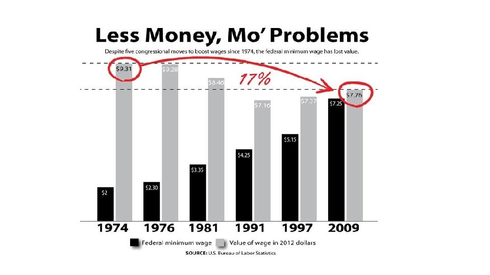
$7. 25 (2009)

Minimum wages around the world*

Adjusting for purchasing power changes the story a little….

Minimum wage laws vary by state….

In 2011, 77 million American workers age 16 and over were paid at hourly rates, representing around 50 percent of all wage and salary workers. • 16 million hourly workers (20% of hourly workers) earn less than the proposed $15 per hour • 1. 3 million (1. 5% of hourly workers) earned exactly the prevailing Federal minimum wage of $7. 25 per hour. • About 1. 7 million (2% of hourly workers) million had wages below the minimum ($2. 13/hr. is the minimum wage for tipped employees). Source: Department of Labor

Most minimum wage workers are part time 20 Percent of minimum wage workers 18 16 14 12 10 8 6 4 2 0 0 to 4 hours 5 to 9 hours 10 to 14 hours 15 to 19 hours 48% 20 to 24 hours 25 to 29 hours 30 to 34 hours 35 to 39 hours 40 hours 41 + hours vary Source: Department of Labor

12 companies with most minimum-wage workers Darden Restaurants Yum Brands Dine. Equity

Highest wage retail companies $11. 27/hr. $9. 67/hr $13. 38/hr $10. 20/hr $9. 67/hr $11/hr $9. 24/hr $9. 48/hr $9. 32/hr $9. 38/hr

Costco's CEO, Craig Jelinek, has publicly endorsed raising the federal minimum wage to $10. 10 an hour, and he takes that to heart. The company's starting pay is $11. 50 per hour, and the average employee wage is $21 per hour, not including overtime.

What effect will a minimum wage hike have on corporate profits? Will a minimum wage hike cause higher prices? Will a minimum wage hike create a rise in unemployment?

Lets try something…. suppose that I were to estimate a production function for the US Economy Cobb-Douglas Production SUMMARY OUTPUT Regression Statistics Multiple R. 99856 R Square. 99712 Gross Domestic Product Capital Stock Labor Force Adjusted R Square . 99702 Standard Error . 03297 Observations 65 ANOVA df Estimated Production Function Regression Residual Total Intercept LN Capital LN Labor 2. 00 64. 00 SS 23. 29 0. 07 23. 36 Coefficient Standard s Error -9. 99 0. 30 0. 62 0. 05 0. 73 0. 09 MS 11. 64 0. 00 t Stat -33. 27 13. 60 8. 03

So, my estimated production function looks something like this So, the economy should be paying. 45% of all income to capital owners and 54% to labor if its acting optimally 70 Actual 65 We are a bit off when compared to actual expenditures 60 55 ? ? ? Estimated Range 50 45 40 1947 1952 1957 1962 1967 1972 1977 1982 1987 1992 1997 2002 2007 2012 Estimated

So if this is the estimated production function, let’s see the implications for a wage hike… Current Minimum Wage: $7. 25 Proposed Minimum Wage: $15 Effect of rising wage on Labor Demand Capital Demand Marginal Cost Marginal costs rise by 58%! Labor demand falls by 49% and businesses replace workers with machines!

In 2011, 77 million American workers age 16 and over were paid at hourly rates, representing around 50 percent of all wage and salary workers. • 16 million hourly workers (20% of hourly workers) earn less than the proposed $15 per hour • 1. 3 million (1. 5% of hourly workers) earned exactly the prevailing Federal minimum wage of $7. 25 per hour. • About 1. 7 million (2% of hourly workers) million had wages below the minimum ($2. 13/hr. is the minimum wage for tipped employees). So, there around 17 million workers that make between $7. 25 and $15 per hour…. Labor demand falls by 49% and businesses replace workers with machines! Our current unemployment rate is 4. 9%. . . if these numbers hold… If the 8. 3 million continue to look for work If the 8. 3 million drop out of the workforce

What about the effect on prices? High Elasticity Low elasticity Prices do not rise much Profits will be fall dramatically Prices rise dramatically Profits will be relatively unaffected If we choose something in the middle

Source: Heritage Foundation