FIN 30210 Managerial Economics Statistical Analysis Part I

FIN 30210: Managerial Economics Statistical Analysis

Part I: Probability The Cubs have a 12% chance of winning the world series this year Here are the odds for Blackjack…. remember, what happens in Vegas stays in Vegas Probability is about having the truth

“Patriots have no need for probability, win coin flip at impossible clip” (Nov. 4 th, 2015) “Belichick has also been extremely lucky. The Pats have won the coin toss 19 of the last 25 times, according to the Boston Globe's Jim Mc. Bride. ” So, what are the odds that the Patriots can win at least 19 out of 25 flips?

To do this, we need a probability distribution…for a coin toss, we have the following. Probability Side Note: 50 Super Bowl Coin Tosses Heads: 24 (48%) Tails: 26 (52%) 1/2 Head Tail Outcome So, suppose that we wanted the odds that the Patriots got 19 wins in a row…. Probability ( A and B) = Probability(A) * Probability (B)

Probability ( A and B) = Probability(A) * Probability (B) Probability 1/2 Head Tail Outcome So, we want the probability of 19 Wins The odds of dying from an asteroid collision with earth in the next 100 years is 1 in 500, 000 (. 000191% - 1 in 523, 560) This isn’t really what we want though…getting 19 wins in a row is one of many ways to get 19 out of 25

What are the odds that the Patriots get 24 out of 25 wins Probability ( A and B) = Probability(A) * Probability (B) Probability ( A or B) = Probability(A) + Probability (B) There are LOTS of ways to get exactly 24 out of 25 wins One way would be L W W W W W W One way would be 24 Wins (. 00000298%) W L W W W W W W 23 Wins (. 00000298%)

What are the odds that the Patriots get 24 out of 25 wins Probability ( A and B) = Probability(A) * Probability (B) Probability ( A or B) = Probability(A) + Probability (B) In Fact, there are 25 ways to get 24 out of 25 wins, so the answer would be (. 000075% - 1 in 1. 3 million) The odds of becoming a movie star are 1 in 1. 5 million

The probability for a number of wins out of a certain number of tries is given by a binomial distribution: k successes in n tries. Probability of success is p Note: 24 out of 25 wins So, the probability that the patriots get EXACTLY 19 out of 25 wins would be (. 52% - 1 in 192) So, the probability that the patriots get AT LEAST 19 out of 25 wins would be The odds of Notre Dame winning the national title in football this year are 1 in 40 (. 73% - 1 in 137)

Here’s the binomial distribution for 25 tosses 18 Odds of 12 or Less = 50% 16 14 Probability (%) 12 10 8 6 4 2 0 0 1 2 3 4 5 6 7 8 9 10 11 12 13 14 15 16 17 18 19 20 21 22 23 24 25 31% . 73%

On the other side of the proverbial coin is losing the toss a lot. In 2011, the Cleveland Browns lost 11 in a row. (. 049% 1 in 2040) The odds of fatally slipping in the shower are 1 in 2500 In 2012, the Carolina Panthers lost 12 in a row. (. 024% - 1 in 4, 166) The odds of getting a hole in 1 in golf are 1 in 5, 000

What are your odds of winning at craps? Easiest Bet – Playing the Pass Line

The Game of Craps – Playing the Pass Line • • • If you roll a 2, 3, or 12, you lose “crap out” If you roll a 7 or 11, you “win” If you roll a 4, 5, 6, 8, 9, 10 the rolled number becomes the “point” If you roll the point, you win, if you roll a seven before rolling the “point” you lose. The Pass Line Pays Even Odds Probability 1/6 Number 1 2 3 4 5 Total on 2 dice Combinations Probability Percentage 2 1+1 1/36 3% 3 1+2, 2+1 2/36 6% 4 1+3, 2+2, 3+1 3/36 8% 5 1+4, 2+3, 3+2, 4+1 4/36 11% 6 1+5, 2+4, 3+3, 4+2, 5+1 5/36 14% 7 1+6, 2+5, 3+4, 4+3, 5+2, 6+1 6/36 17% 8 2+6, 3+5, 4+4, 5+3, 6+2 5/36 14% 9 3+6, 4+5, 5+4, 6+3 4/36 11% 10 4+6, 5+5, 6+4 3/36 8% 11 5+6, 6+5 2/36 6% 12 6+6 1/36 3% 6

Come Out • Win = 23% • Lose = 12% • Roll Again = 65% • 4 or 10 = 16% • 5 or 9 = 22% • 6 or 8 = 27% 18 16 14 Probability (%) 12 10 8 6 4 2 0 2 3 “Craps” (9%) 4 5 “Point” (33%) 6 7 8 “Win” (17%) 9 10 11 12 “Craps” (3%) “Point” (33%) “Win” (6%)

65 Percent of the time, you have a “point” to make Come Out = 4, 10 Next Roll • Win = 8% • Lose = 17% • Roll Again = 75% Come Out = 6, 8 Next Roll • Win =14% • Lose = 17% • Roll Again = 69% 17% 16 Probability (%) Come Out = 5, 9 Next Roll • Win =11% • Lose = 17% • Roll Again = 72% 18 14% 14 14% 11% 12 11% 10 8% 8% 8 6% 6 4 16% 3% 3% 2 0 2 3 4 5 6 7 8 9 10 11 12

So, what's the probability that you win with a pass bet? Total on 2 dice Probability Roll a Seven 6/36 Roll a 11 2/36 Roll a 4 and then roll another 4 before rolling a 7 (3/36)*PR(4 before a 7) Roll a 5 and then roll another 5 before rolling a 7 (4/36)*PR(5 before a 7) Roll a 6 and then roll another 6 before rolling a 7 (5/36)*PR(6 before a 7) Roll a 8 and then roll another 8 before rolling a 7 (5/36)*PR(8 before a 7) Roll a 9 and then roll another 9 before rolling a 7 (4/36)*PR(9 before a 7) Roll a 10 and then roll another 10 before rolling a 7 (3/36)*PR(10 before a 7) These are a bit tricky…. .

What’s the probability the you roll a 4 before you roll a 7? Total on 2 dice Probability 4 3/36 7 6/36 All Other #s 27/36 A useful bit of math Roll a 4 Roll something other than a 4 or 7, then roll a 4 Roll something other than a 4 or 7 twice, then roll a 4 Roll something other than a 4 or 7 three times, then roll a 4

So, what's the probability that you win with a pass bet? Event Probability Total on 2 dice Probability Percentage (approx. ) 4 before a 7 3/9 Roll a Seven 6/36 16. 67% 5 before a 7 4/10 Roll a 11 2/36 5. 56% 6 before a 7 5/11 Roll a 4 and then roll another 4 before rolling a 7 (3/36)*(3/9) = 9/324 2. 78% 8 before a 7 5/11 Roll a 5 and then roll another 5 before rolling a 7 (4/36)*(4/10) = 16/360 4. 44% 9 before a 7 4/10 Roll a 6 and then roll another 6 before rolling a 7 (5/36)*(5/11) = 25/396 6. 31% 10 before a 7 3/9 Roll a 8 and then roll another 4 before rolling a 8 (5/36)*(5/11) = 25/396 6. 31% Roll a 9 and then roll another 9 before rolling a 7 (4/36)*(4/10) = 16/360 4. 44% Roll a 10 and then roll another 10 before rolling a 7 (3/36)*(3/9) = 9/324 2. 78% Total 244/495 49. 3%

The Game of Craps – Playing the Pass Line • • • If you roll a 2, 3, or 12, you lose “crap out” If you roll a 7 or eleven, you win “win” If you roll a 4, 5, 6, 8, 9, 10 the rolled number becomes the “point” If you roll the point, you win, if you roll a seven before rolling the “point” you lose. The Pass Line Pays even odds Playing the Pass Line This is known as the “House Edge” Win = 49. 3% - Loss = 50. 7% -1. 4% “The Gambler’s Ruin” A gambler playing a negative expected value game will eventually go broke with probability one!! Event Probability (approx. ) Pass Line Win 22. 2% Pass Line Loss 11. 1% 4, or 10 Win 5. 6% 4 or 10 Loss 11. 1% 5 or 9 Win 8. 9% 5 or 9 Loss 13. 3% 6 or 8 Win 12. 6% 6 of 8 Loss 15. 2%

The Game of Craps – Playing the Pass Line If you roll a 2, 3, or 12, you lose “crap out” If you roll a 7 or eleven, you win “win” If you roll a 4, 5, 6, 8, 9, 10 the rolled number becomes the “point” If you roll the point, you win, if you roll a seven before rolling the “point” you lose. • The Pass Line Pays even odds • • Playing the Pass Line Expected Value measures the average outcome over a large number of attempts, given the probabilities of each outcome. Event Probability (approx. ) Pass Line Win 22. 2% Pass Line Loss 11. 1% 4, or 10 Win 5. 6% 4 or 10 Loss 11. 1% 5 or 9 Win 8. 9% 5 or 9 Loss 13. 3% 6 or 8 Win 12. 6% 6 of 8 Loss 15. 2%

Playing the Pass Line Expected Percentage loss (House Edge) For a $1 Pass Bet Event Probability Total Bet Payout Expected Total Bet Pass Line Win 22. 22% $1 . 222 Pass Line Loss 11. 11% $1 -. 111 4, or 10 Win 5. 56% $1 . 392 . 0556 4 or 10 Loss 11. 11% $1 -$1 -. 444 . 1111 5 or 9 Win 8. 89% $1 . 623 . 0889 5 or 9 Loss 13. 33% $1 -. 665 . 1333 6 or 8 Win 12. 63% $1 . 882 . 1263 6 of 8 Loss 15. 15% $1 -. 912 . 1515 -. 0141 1. 00 Total 100%

Suppose that the first roll is a 4. I can now make an additional bet. I can make a bet that a 4 is rolled before a 7. This is called “Playing the odds” Event Probability 4 before a 7 3/9 5 before a 7 4/10 6 before a 7 5/11 8 before a 7 5/11 9 before a 7 4/10 10 before a 7 3/9 Bet Payout 4 or 10 2 to 1 5 or 9 3 to 2 6 or 8 6 to 5 The house pays odds equal to the true odds, so the house edge on this additional bet are ZERO!!!!!!! This is the only fair bet in Vegas!!!

Suppose that you can bet twice your initial bet on the odds Whatever your initial Pass/Don’t Pass Wager, you can up your bet on a point as follows • You can bet 2 X your initial bet if your point is 4 or 10 (Pays 2 to 1) • You can bet 2 X your initial bet if your point is 5 or 9 (Pays 3 to 2) • You can bet 2 X your initial bet if your point is 6 or 8 (Pays 6 to 5) For a $1 Initial Bet – Playing Pass/w 2 x odds Event Probability Total Bet Payout Expected Bet Pass Line Win 22. 22% $1 . 222 Pass Line Loss 11. 11% $1 -. 111 4, or 10 Win (Pays 2 -1) 5. 56% $3 $5 . 392 . 167 4 or 10 Loss 11. 11% $3 -$3 -. 444 . 333 5 or 9 Win (Pays 3 -2) 8. 89% $3 $4 . 623 . 267 5 or 9 Loss 13. 33% $3 -. 665 . 400 6 or 8 Win (Pays 6 -5) 12. 63% $3 $3. 40 . 882 . 379 6 of 8 Loss 15. 15% $3 -. 912 . 455 -. 0141 2. 33 Total 100% Expected Percentage loss (House Edge) The expected loss is the same, but your overall bet is bigger, so the percentage loss is smaller!!

A Common Casino Betting System for Casino Craps is the “ 3 -4 -5” System Whatever your initial Pass/Don’t Pass Wager, you can up your bet on a point as follows • You can bet 3 X your initial bet if your point is 4 or 10 (Pays 2 to 1) • You can bet 4 X your initial bet if your point is 5 or 9 (Pays 3 to 2) • You can bet 5 X your initial bet if your point is 6 or 8 (Pays 6 to 5) For a $1 Initial Bet – Playing Pass/w 3 -4 -5 odds Event Probability Total Bet Payout Expected Bet Pass Line Win 22. 22% $1 . 222 Pass Line Loss 11. 11% $1 -. 111 4, or 10 Win (Pays 2 -1) 5. 56% $4 $7 . 392 . 224 4 or 10 Loss 11. 11% $4 -$4 -. 444 5 or 9 Win (Pays 3 -2) 8. 89% $5 $7 . 623 . 444 5 or 9 Loss 13. 33% $5 -. 665 . 666 6 or 8 Win (Pays 6 -5) 12. 63% $6 $7 . 882 . 7578 6 of 8 Loss 15. 15% $6 -. 912 . 909 -. 0141 3. 77 Total 100% Expected Percentage loss (House Edge) The bigger the multiple allowed, the smaller the house edge!!

House Edge for other craps bets Bet House Edge Pass/Come 1. 41% Don’t Pass/Don’t Come 1. 36% Pass/Come(2 X odds) . 606% Don’t Pass/Don’t Come (2 X odds) . 466% Place 6 and 8 1. 52% Place 5 and 9 4. 00% Place 4 and 10 6. 67% Buy 6 and 8 4. 76% Buy 5 and 9 4. 76% Buy 4 and 10 4. 76% Lay 6 or 8 4. 00% Lay 5 or 9 3. 23% Lay 4 or 10 2. 44% Field Bet 5. 56% Any Craps 11. 11% 6 or 8 Hard way 9. 09% 4 or 10 Hard way 11. 10% 11 or 3 11. 10% 2 or 12 13. 90% Any 7 16. 70%

Here’s a comparison of casino edges on other games… Craps Other Games House Edge when you Take the Odds Game House Edge (w/ proper play) Table Odds Taken Pass Line Don’t Pass Blackjack 0. 5% 0 x 1. 41% 1. 36% Video Poker 0. 5% - 5% 1 x 0. 848% 0. 682% Baccarat 1. 06% 2 x 0. 606% 0. 455% Roulette 5. 5% 3 x 0. 471% 0. 341% Slot Machines 0% – 17% 3 -4 -5 x 0. 374% 0. 273% Progressive Slots 5% -17% 5 x 0. 326% 0. 227% Keno 25%+ 10 x 0. 184% 0. 124% Typical State Lottery 50%+ 20 x 0. 099% 0. 065% 100 x 0. 021% 0. 014%

What are the odds that it will be 80 degrees tomorrow in South Bend? As with the first two examples, this involves a probability distribution

Just as with the coin flip or the dice roll, we can imagine a “truth” out there governing South Bend temperatures. This “truth”, again, is in the form of a probability distribution. Probability Temperature

Probability 0. 2% We can use the normal distribution to get the probability that the temperature lies within various ranges 2. 3% 34% 13. 5% 2. 3% 0. 2% Temperature 68% 95% 99. 6%

So, for example…… Probability 0. 2% 34% 2. 3% 34% 13. 5% Temperature Range Probability <15 0. 2% 15 – 30 2. 3% 30 – 45 13. 5% 45 – 60 34% 60 – 75 34% 75 – 90 13. 5% 90 – 105 2. 3% >105 . 2% 2. 3% 13. 5% 0. 2% Temperature 68% 95% 99. 6%

Conditional distributions give us probabilities conditional on some observable information What is the probability that the Temperature in south bend is greater than 15 degrees Probability Unconditional Conditional on February Temp 99. 8% Temp 16%

Part II: Statistics is about finding the truth

Law of large numbers: In statistics, as the number of identically distributed, randomly generated variables increases, their sample mean (average) approaches their theoretical mean. The law of large numbers was first proved by the Swiss mathematician Jakob Bernoulli. Number of data points increases Jakob Bernoulli 1655 - 1705 (Population Mean) (Population Variance)

Average Monthly Temperatures in Indiana from 1894 - 2016 Sample Statistics • Average = 50. 7 • Std. Dev. = 16. 3 • High = 78. 1 • Low = 22. 1 We have Average Monthly temperatures (1894 – 2016) for 36 locations across Indiana. This is what we would call a “cross sectional” dataset (multiple observations at a single point in time)

Sample Statistics • Average = 50. 7 • Std. Dev. = 16. 3 • High = 78. 1 • Low = 22. 1 4. 5 4 3. 5 Frequency (%) 3 2. 5 2 1. 5 1 0. 5 0 20 25 30 35 40 45 50 55 60 65 70 75 80 85

Suppose that we condition on “Northern Indiana” or “Southern Indiana” Sample Statistics • Average = 47. 9 • Std. Dev. = 16. 8 • High = 72. 6 • Low = 22. 1 We have Average Monthly temperatures (1894 – 2016) for 36 locations across Indiana. This is what we would call a “cross sectional” dataset (multiple observations at a single point in time)

“Northern Indiana” 7 Frequency (%) 6 Sample Statistics • Average = 47. 9 • Std. Dev. = 16. 8 • High = 72. 6 • Low = 22. 1 5 4 3 2 1 0 20 25 30 35 40 45 50 55 60 65 70 75 80 85 “Southern Indiana” 7 Frequency (%) 6 Sample Statistics • Average = 53. 1 • Std. Dev. = 15. 7 • High = 78. 1 • Low = 24. 2 5 4 3 2 1 0 20 25 30 35 40 45 50 55 60 65 70 75 80 85

January - March 14 Frequency (%) 12 Sample Statistics • Average = 32. 7 • Std. Dev. = 6. 5 • High = 47. 5 • Low = 22. 1 10 8 6 4 2 0 20 25 30 35 40 18 45 50 55 60 65 70 75 80 85 Temperature I could also condition on Month(s) of the year June - August Frequency (%) 16 14 Sample Statistics • Average = 70. 8 • Std. Dev. = 2. 6 • High = 78. 8 • Low = 65. 1 12 10 8 6 4 2 0 20 25 30 35 40 45 50 55 60 65 70 75 80 85 Temperature

February Frequency (%) 25 20 Sample Statistics • Average = 32. 7 • Std. Dev. = 3. 5 • High = 37. 7 • Low = 23. 6 15 10 5 0 20 25 30 35 40 20 50 55 60 65 70 75 80 Or individual months of the year July 18 Frequency (%) 45 85 Temperature 16 Sample Statistics • Average = 72. 6 • Std. Dev. = 1. 9 • High = 78. 1 • Low = 69. 0 14 12 10 8 6 4 2 0 20 25 30 35 40 45 50 55 60 65 70 75 80 85 Temperature

Northern Indiana in February 35 30 Sample Statistics • Average = 25. 9 • Std. Dev. = 1. 4 • High = 27. 4 • Low = 23. 6 25 20 15 10 5 Or individual months of the year and locations 0 20 25 30 35 35 40 45 50 55 60 65 70 75 80 85 Northern Indiana in July 30 Sample Statistics • Average = 70. 8 • Std. Dev. = 1. 1 • High = 72. 6 • Low = 69. 0 25 20 15 10 5 0 20 25 30 35 40 45 50 55 60 65 70 75 80 85

For Indiana Probability “I’m 95% sure that the temperature for September will be between 18 and 83 degrees” 0. 2% 34% 2. 3% 34% 13. 5% 2. 3% 13. 5% 0. 2% Temperature 68% 95% 99. 6%

So, for example……for Northern Indiana in September Sample Statistics Probability “I’m 95% sure that the temperature for September will be between 60 and 64 degrees” 0. 2% 34% 2. 3% 34% 13. 5% 2. 3% 13. 5% 0. 2% Temperature 68% 95% 99. 6%

Regressions are about estimating conditional distributions Linear Regressions make several key assumptions • • • Linear Relationship Multivariate Normality No or Little Multicollinearity No Auto-correlation Homoscedasticity Independent Variable Error Term Explained Variable Parameters to be estimated

Frequency Conditional Distribution of Y

The OLS (Ordinary Least Squares) method estimates the parameters alpha and beta by minimizing the sum of squared errors. Estimated Coefficients

We also have a set of error terms Frequency These errors are a sampling of the population of errors

Each regression gives us a sample of the distribution of errors (not the entire population of errors). Therefore, the estimated coefficients are not the true coefficients, but rather, they are samples drawn from a distribution of possible true parameter values Frequency

A few important things regarding these parameter estimates… The estimated parameters are drawn from a distribution with a mean equal to the true parameter value – we are not making biased prediction! These parameters are unknown, so we need to estimate them from the data 1) The variance of the parameters is smaller (the estimates are more precise)when the variance of x is large 2) As the number of observations gets large, the variance approaches zero – we learn the truth!

Law of large numbers: In statistics, as the number of identically distributed, randomly generated variables increases, their sample mean (average) approaches their theoretical mean. The law of large numbers was first proved by the Swiss mathematician Jakob Bernoulli. Sample Estimates Population Parameters Number of observations gets big

We also have some additional “diagnostics” to check the performance of the regression Total Sum of Squares = Total Variation in the Data we are trying to explain Regression Sum of Squares + Total Variation in the data we have actually Residual Sum of Squared Residuals Total Variation in the Data left unexplained Standard Error of the Regression R Squared of the Regression The percentage of the variation of Y explained in the regression The is the average error of our estimates

If we would like to make a forecast using our regression data, we need to calculate the conditional distribution Frequency 1) Note that since our estimates are unbiased, our forecasts will also be unbiased! 2) As our sample size gets bigger, the variance of our forecasts goes down (our forecasts get more precise) 3) If the variance of X is big, we get better forecasts

A forecast is only as good as the error attached to it!!! 95% Confidence Interval We always get the best forecast at the sample average

Example: Does the striped ground cricket chirp differently at different temperatures? Temperature (F) 20. 0 88. 6 16. 0 71. 6 19. 8 93. 3 18. 4 84. 3 17. 1 80. 6 15. 5 75. 2 14. 7 69. 7 17. 1 82. 0 15. 4 69. 4 16. 2 83. 3 15. 0 79. 6 17. 2 82. 6 16. 0 80. 6 17. 0 83. 5 14. 4 76. 3 24. 0 22. 0 Chirps/Sec. Chirps Per Sec 20. 0 18. 0 16. 0 14. 0 12. 0 10. 0 65. 0 70. 0 75. 0 80. 0 85. 0 Temperature (F) 90. 0 95. 0

Example: Does the striped ground cricket chirp differently at different temperatures? Temperature (F) 20. 0 88. 6 16. 0 71. 6 19. 8 93. 3 18. 4 84. 3 17. 1 80. 6 15. 5 75. 2 14. 7 69. 7 17. 1 82. 0 15. 4 69. 4 16. 2 83. 3 15. 0 79. 6 17. 2 82. 6 16. 0 80. 6 17. 0 83. 5 14. 4 76. 3 24. 0 22. 0 Chirps/Sec. Chirps Per Sec 20. 0 18. 0 16. 0 14. 0 12. 0 10. 0 65. 0 70. 0 75. 0 80. 0 85. 0 Temperature (F) 90. 0 95. 0

Chirps Per Sec Temperature (F) 20. 0 88. 6 3. 3 8. 6 28. 6 73. 3 16. 0 71. 6 -0. 7 -8. 4 5. 5 71. 2 19. 8 93. 3 3. 1 13. 3 41. 7 175. 8 18. 4 84. 3 1. 7 4. 3 7. 4 18. 1 17. 1 80. 6 0. 4 0. 6 0. 3 15. 5 75. 2 -1. 2 -4. 8 5. 6 23. 4 14. 7 69. 7 -2. 0 -10. 3 20. 2 106. 9 17. 1 82. 0 0. 4 2. 0 0. 9 3. 8 15. 4 69. 4 -1. 3 -10. 6 13. 3 113. 2 16. 2 83. 3 -0. 5 3. 3 -1. 5 10. 6 15. 0 79. 6 -1. 7 -0. 4 0. 7 0. 2 17. 2 82. 6 0. 5 2. 6 1. 4 6. 6 16. 0 80. 6 -0. 7 0. 6 -0. 4 0. 3 17. 0 83. 5 0. 3 3. 5 1. 2 12. 0 14. 4 76. 3 -2. 3 -3. 7 8. 4 14. 0 Average = 16. 7 Average = 80. 0 Sum=133. 5 Sum =629. 8

Chirps Per Sec Temperature (F) Predicted Error Squared Error 20. 0 88. 6 18. 5 -1. 5 2. 3 16. 0 71. 6 14. 9 -1. 1 1. 3 19. 8 93. 3 19. 5 -0. 3 0. 1 18. 4 84. 3 17. 6 -0. 8 0. 7 17. 1 80. 6 16. 8 -0. 3 0. 1 15. 5 75. 2 15. 6 0. 1 0. 0 14. 7 69. 7 14. 5 -0. 2 0. 1 17. 1 82. 0 17. 1 0. 0 15. 4 69. 4 14. 4 -1. 0 16. 2 83. 3 17. 3 1. 1 1. 3 15. 0 79. 6 16. 6 1. 6 2. 4 17. 2 82. 6 17. 2 0. 0 16. 0 80. 6 16. 8 0. 6 17. 0 14. 4 83. 5 76. 3 17. 4 15. 9 0. 4 1. 5 0. 1 2. 1 Average = 16. 7 Average = 80. 0 Variance = 2. 89 Variance = 44. 98 Sum = 12. 3

Actual Total Sum of Squares Predicted 20. 0 18. 5 11. 2 3. 3 2. 3 16. 0 14. 9 0. 4 3. 2 1. 3 19. 8 19. 5 9. 9 7. 9 0. 1 18. 4 17. 6 3. 1 0. 8 0. 7 17. 1 16. 8 0. 2 0. 0 0. 1 15. 5 15. 6 1. 3 1. 1 0. 0 14. 7 14. 5 3. 8 4. 8 0. 1 17. 1 0. 2 0. 0 15. 4 14. 4 1. 6 5. 1 1. 0 16. 2 17. 3 0. 2 0. 5 1. 3 15. 0 16. 6 2. 7 0. 0 2. 4 17. 2 0. 3 0. 0 16. 8 0. 4 0. 0 0. 6 17. 0 14. 4 17. 4 15. 9 0. 1 5. 1 0. 5 0. 6 0. 1 2. 1 Sum = 28. 3 Sum = 12. 3 Average = 16. 7 Sum = 40. 6 Regression Sum of Squares R Squared of the Regression Standard Error of the Regression

24. 0 95% Confidence Interval 17. 7+/-2(1. 85) = [21. 4, 14] 20. 0 17. 7 Chirps/Sec. So, lets calculate a prediction for the number of chirps at a temperature of 85 degrees 22. 0 18. 0 16. 0 14. 0 12. 0 10. 0 65. 0 70. 0 75. 0 80. 0 85. 0 Temperature (F) 90. 0 95. 0

Here are the results of the regression done in Excel SUMMARY OUTPUT Regression Statistics Multiple R R Square Adjusted R Square Standard Error Observations 0. 84 0. 70 0. 67 0. 97 15 ANOVA df Regression Residual Total SS 1 13 14 Intercept Temperature (F) Coefficients -0. 31 0. 21 MS 28. 29 12. 27 40. 56 Standard Error 3. 11 0. 04 F 28. 29 0. 94 29. 97 t Stat P-value -0. 10 5. 47 Significance F 0. 00 0. 92 0. 00 Lower 95% -7. 02 0. 13 Upper 95% 6. 41 0. 30

How does taking LSD affect your performance on a math test? 90 80 70 Test Score 60 50 40 30 20 “Correlation of performance test scores with “tissue concentration” of Lysergic Acid Diethylamide in human subjects” John Wagner, George Aghajanian, and Oscar Bing March 22, 1968 10 0 1 2 3 4 Tissue Concentration 5 6 7

How does taking LSD affect your performance on a math test? SUMMARY OUTPUT Regression Statistics Multiple R R Square Adjusted R Square Standard Error 0. 963 0. 927 0. 912 5. 710 Observations 7. 000 ANOVA Regression Residual 1 5 SS 2056. 44358 163. 0445059 Total 6 2219. 488086 Intercept Tissue Conc (x) df Coefficients 90. 29465244 Standard Error 5. 647752669 -9. 565531392 1. 204533226 MS F 2056. 44358 63. 06387 32. 60890117 Significanc e F 0. 00051 Lower Upper t Stat P-value Lower 95% Upper 95% 95. 0% 15. 98771365 1. 74 E-05 75. 77664 104. 8127 -7. 941276492 0. 00051 -12. 6619 -6. 46918

What would your predicted score be with a concentration of 4? 90 Mean x = 4. 3 Var(x) = 3. 7 80 70 Test Score 60 50 40 30 20 10 0 95% Confidence Interval 51. 9 +/- 12. 2 64. 1, 39. 7 1 2 3 4 Tissue Concentration 5 6 7

What about the possibility of a non-linear relationship between LSD usage and math performance? VS Beta measures the unit change in test score per unit change in LSD concentration Beta measures the percentage change in test score per unit change in LSD concentration

Both functional forms indicate a negative relationship, but one is linear while the other is non-linear 120 100 80 60 40 20 0 0 1 2 3 4 5 6 7

I can estimate this nonlinear relationship through a transformation of variable? Take the natural log of both sides… A little math here… Define a new constant…

How does taking LSD affect your performance on a math test? SUMMARY OUTPUT Regression Statistics Multiple R R Square Adjusted R Square Standard Error Observations 0. 961663013 0. 924795751 0. 909754901 0. 114937569 7 ANOVA Regression Residual Total Intercept Tissue Conc (x) df 1 5 6 Coefficients 4. 648346245 -0. 19010758 SS 0. 812264483 0. 066053224 0. 878317707 Standard Error 0. 113676212 0. 024244471 Significan F ce F 61. 4856 0. 000541 MS 0. 812264483 0. 013210645 Lower Upper t Stat P-value 95% 95. 0% 40. 89110775 1. 65 E-07 4. 356132 4. 94056 -7. 841275714 0. 000541 -0. 25243 -0. 12779

What would your predicted score be with a concentration of 4? 90 Mean x = 4. 3 Var(x) = 3. 7 80 Test Score 70 60 50 40 30 20 12. 2% 10 0 95% Confidence Interval 48. 4 +/- 24. 4% 1 2 3 4 Tissue Concentration 60. 2, 36. 6 5 6 7

A linear regression capture several different non-linear relationships by transforming the variables! Functional Form Regression Equation Interpretation A one unit change in X causes a Beta units change in Y A one unit change in X causes a Beta percent change in Y A one percent change in X causes a Beta units change in Y A one percent change in X causes a Beta percent change in Y

“Northern Indiana” 7 Sample Statistics • Average = 47. 9 • Std. Dev. = 16. 8 6 Frequency (%) 5 4 3 2 1 0 20 25 30 35 40 45 50 55 60 65 70 75 80 85 Indiana 4. 5 Sample Statistics • Average = 50. 7 • Std. Dev. = 16. 3 4 Frequency (%) 3. 5 3 2. 5 2 1. 5 1 0. 5 0 20 25 30 35 40 45 50 55 60 65 70 75 80 85 I could accomplish the same thing with a “temperature dummy”

Distribution for Northern Indiana SUMMARY OUTPUT Regression Statistics Multiple R 0. 107015815 R Square 0. 011452385 Adjusted R Square Standard Error Mean x =. 28 Var(x) =. 20 Average Temperature for “Not Northern Indiana” 0. 009153437 16. 22029062 Observations 432 ANOVA Regression Residual Total Intercept North df 1 430 SS 1310. 641907 113132. 0659 431 114442. 7079 MS 1310. 641907 263. 0978278 F 4. 981576314 Significance F 0. 026133096 Coefficients 51. 79651334 Standard Error 0. 918293128 t Stat 56. 40520632 P-value 8. 0168 E-201 Lower 95% 49. 99161169 Upper 95% 53. 60141498 -3. 888803317 1. 742338706 -2. 231944514 0. 026133096 -7. 313363408 -0. 464243226

“Southern Indiana” 7 Frequency (%) 6 5 Sample Statistics • Average = 53. 1 • Std. Dev. = 15. 7 4 3 2 1 0 20 25 30 35 40 45 50 55 60 65 70 75 80 Indiana 4. 5 4 Sample Statistics • Average = 50. 7 • Std. Dev. = 16. 3 3. 5 Frequency (%) 85 3 2. 5 2 1. 5 1 0. 5 0 20 25 30 35 40 45 50 55 60 65 70 75 80 85 Suppose that I repeat the process for Southern Indiana

Distribution for Northern Indiana Mean x =. 39 Var(x) =. 24 SUMMARY OUTPUT Regression Statistics Multiple R 0. 114475818 R Square 0. 013104713 Adjusted R Square 0. 010809608 Standard Error 16. 20672908 Observations 432 Average Temperature for “Not Southern Indiana” ANOVA Regression Residual Total Intercept South df 1 430 431 Coefficients 49. 22994863 3. 822021173 SS 1499. 738841 112942. 969 114442. 7079 Standard Error 0. 997455223 1. 59948673 MS 1499. 738841 262. 6580675 F 5. 709852566 t Stat 49. 35554748 2. 389529779 Significance F 0. 017299906 P-value 3. 1797 E-179 0. 017299906 Lower 95% 47. 26945418 0. 678236097 Upper 95% 51. 19044307 6. 96580625

Northern Indiana Southern Indiana SUMMARY OUTPUT Average Temperature for Central Indiana Regression Statistics Multiple R 0. 134093809 R Square 0. 017981149 Adjusted R Square 0. 013402973 Standard Error 16. 18547051 Observations 432 ANOVA Regression Residual Total Intercept North South df 2 429 431 Coefficients 50. 34616241 -2. 728522571 2. 900701864 SS 2057. 811439 112384. 8964 114442. 7079 Standard Error 1. 255855211 1. 869422778 1. 717587401 MS 1028. 905719 261. 9694555 F 3. 927578951 t Stat 40. 0891456 -1. 459553507 1. 68882344 Significance F 0. 020403391 P-value 3. 6261 E-147 0. 145144669 0. 09197992 Lower 95% 47. 87776753 -6. 402890097 -0. 475231843 Upper 95% 52. 81455728 0. 945844954 6. 27663557

Be mindful of what hypothesis you are testing! Northern Dummy Only (T-stats in parentheses) Northern Indiana has a different average temperature than the rest of the state (-2. 2) Significant Southern Dummy Only (T-stats in parentheses) Northern Indiana has a different average temperature than the rest of the state (2. 4) Significant Northern and Southern Dummy (T-Stats in parentheses) (-1. 5) (-1. 7) Not Significant!!! Northern and Southern Indiana have a different average temperature than central Indiana

Suppose I put in Dummies for all three regions… There is no other region, so we know that One of our assumptions is violated! • • • Linear Relationship Multivariate Normality No or Little Multicollinearity No Auto-correlation Homoscedasticity

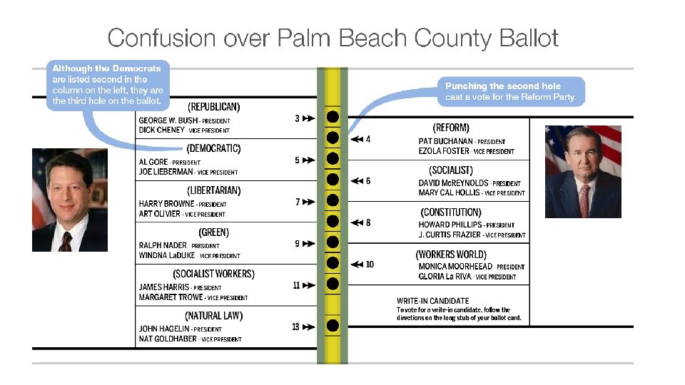
Example: The Famous 2000 Election Al Gore Democrat Pat Buchanan Reform Party George W. Bush Republican Ralph Nader Green Party The Case of Palm Beach County

Overall State Results Candidate Vote Total Percentage George W. Bush 2, 909, 815 49. 039 Al Gore 2, 909, 578 49. 035 Ralph Nader 96, 844 1. 633 Pat Buchanan 17, 358 . 293 Total 5, 933, 595 100. 000 Palm Beach County Results Candidate Vote Total Percentage George W. Bush 152, 954 35. 44 Al Gore 269, 696 62. 48 Ralph Nader 5, 564 1. 29 Pat Buchanan 3, 407 . 79 Total 431, 621 100. 00 Did Pat Buchanan REALLY get 3, 407 votes in Palm Beach County

The Strategy: Use available data on demographics from the counties in Florida (omitting Palm Beach County) to estimate a relationship between demographics and Pat Buchanan's vote total “Are a function of” Pat Buchanan’s Votes Demographic Statewide Average Palm Beach % Black 15. 9% 14. 4% % Hispanic 6. 3% 9. 8% % Over 65 yrs. 16. 9% 23. 7% % College Degree 13. 9% 22. 1% Income (in thousand) 26. 188 33. 518 Observable Demographics Using Palm Beach demographics, forecast Pat Buchanan’s vote total for Palm Beach

Turns out, the best fitting regression was as follows Buchanan Votes Total Votes *100 Variable Coefficient Standard Error t - statistic Intercept 2. 146 . 396 5. 48 Black (%) -. 0132 . 0057 -2. 88 Age 65 (%) -. 0415 . 0057 -5. 93 Hispanic (%) -. 0349 . 0050 -6. 08 College (%) -. 0193 . 0068 -1. 99 Income (000 s) -. 0658 . 00113 -4. 58 R Squared =. 73

Demographic Palm Beach % Black 14. 4% % Hispanic 9. 8% % Over 65 yrs. 23. 7% % College Degree 22. 1% Income (in thousand) 33. 518 This would be our prediction for Pat Buchanan’s vote total! +/- 2 Standard Deviation Confidence Interval (25. 56%)

Demographic Palm Beach % Black 14. 4% % Hispanic 9. 8% % Over 65 yrs. 23. 7% % College Degree 22. 1% Income (in thousand) 33. 518 Frequency Event Odds Win the Powerball 1 in 292, 000 Struck by Lightning 1 in 960, 000 Crushed by a Vending Machine 1 in 112, 000 Becoming a Movie Star 1 in 1, 505, 000 Having Identical Quadruplets 1 in 15, 000 7 Standard Deviations from the mean • 1 in 390, 882, 215, 445 +/1 2 Standard Deviations

Speaking of Election, who will win this year’s election? VS Let’s ask Ray Fair…. he should have a pretty good idea!

Democratic Share of Two Party Presidential Vote Variable Ray Fair Yale University The Fair Presidential Election Model Description Coefficient Value (T-Statistic) Constant 47. 75 (79. 15) Average Annual Growth in Real Per Capita GDP (First three quarters of election year) . 667 (5. 79) Average Annual Growth in GDP Deflator (for first 15 quarters of the current administration) -. 690 (-2. 34) # of Quarters of the current administration with annual real GDP per capita growth exceeds 3. 2% . 968 (4. 03) 1 if Democratic incumbent is running again, -1 if Republican incumbent is running again, otherwise, 0 3. 01 (2. 14) 1 (-1) if Democrat (Republican) has been in office for 2 terms. -3. 80 (-3. 10) 0 if ether party in for 1 term 1 If a democrat is the incumbent, -1 if a Republican is the incumbent -1. 56 (-0. 71) R Squared =. 912

Democratic Share of Two Party Presidential Vote Predictors for the 2016 Presidential Election Description Value Average Annual Growth in Real Per Capita GDP (First three quarters of election year) . 87% (Estimated) Average Annual Growth in GDP Deflator (for first 15 quarters of the current administration) 1. 28% # of Quarters of the current administration with annual real GDP per capita growth exceeds 3. 2% 3 Quarters out of 15 1 if Democratic incumbent is running again, -1 if Republican incumbent is running again, otherwise 0 0 (No) 1 (-1) if Democrat (Republican) has been in office for 2 terms. 0 if ether party in for 1 term 1 (2 Terms) Democrat Incumbent 1 (Yes)

Since 1908, the Fair Model has correctly predicted 23 out of 27 elections (85% Success Rate) Election He predicted every Year election between 1960 1908 and 1960 correctly!! Ray Fair Candidates Predicted Democrat Predicted Republican Actual Democrat Actual Republican Kennedy (D) vs. Nixon (R) 51. 3 48. 7 50. 1 49. 9 1964 Johnson (D) vs. Goldwater (R) 55. 3 44. 7 61. 3 38. 7 1968 Humphrey (D) vs. Nixon (R) 49. 0 51 49. 6 50. 4 1972 Mc. Govern (D) vs. Nixon (R) 39. 9 60. 1 38. 2 61. 8 1976 Carter (D) vs. Ford (R) 49. 2 50. 8 51. 1 48. 9 1980 Carter (D) vs. Reagan (R) 46. 6 53. 4 44. 7 55. 3 1984 Mondale (D) vs. Reagan (R) 42. 8 57. 2 40. 1 59. 9 1988 Dukakis (D) vs. Bush (R) 45. 0 55 46. 0 54 1992 Clinton (D) vs. Bush (R) 48. 8 51. 2 53. 6 46. 4 1996 Clinton (D) vs. Dole (R) 53. 2 46. 8 54. 7 45. 3 2000 Gore (D) vs. Bush (R) 49. 3 50. 7 50. 3 49. 7 2004 Kerry (D) vs. Bush (R) 45. 5 54. 5 48. 8 51. 2 2008 Obama (D) vs. Mc. Cain (R) 55. 2 44. 8 53. 7 46. 3 2012 Obama (D) vs. Romney (R) 49. 0 51. 3 48. 7

Democratic Share of Two Party Presidential Vote And the winner is…. . VS 45. 0% 55. 0% Congratulations to President Elect Trump!

Cross Sectional Regressions vs. Time Series Regressions 0 1 2 3 A cross sectional regression focusses on variations across locations (or other factors) at a single point in time 0 1 2 3 A time series regression focusses entirely on variation across time (ignoring variation across location (or other factors)

Luckily, all the tools from the cross-sectional analysis carries over to time series analysis Time indicator (t = 0, 1, 2, 3, 4) All the properties of the estimates are the same!

We can forecast just as we did before as well In Sample The further out into the future you try and predict, the bigger your errors get! The longer your sample period is, the better you do!!

Example: South Bend Daily High Temperature (2013 – 2014) 16 14 Frequency (%) 12 10 8 Sample Statistics • Average = 57. 8 • Std. Dev. = 21. 9 • Median = 60. 1 • Mode = 84 • High = 97 • Low = 1. 2 6 4 2 0 0 5 10 15 20 25 30 35 40 45 50 55 60 65 70 75 80 85 90 95 100 105 Temperature

Here’s the time series representation for Temperature in South Bend 120 100 80 60 40 20 0 1/2013 4/2013 7/2013 10/2013 1/2014 4/2014 7/2014 10/2014

Daily Observations t = 0 is 1/1/2013 SUMMARY OUTPUT Temperature rises by. 01 degrees per day (3. 65 degrees per year)!!! Regression Statistics Multiple R 0. 09 R Square 0. 01 Adjusted R Square 0. 01 Standard Error 21. 82 Observations 730. 00 ANOVA Regression Residual Total Intercept Time df 1. 00 728. 00 729. 00 SS 2934. 51 346550. 24 349484. 76 Coefficients Standard Error 54. 36 1. 61 0. 00 MS 2934. 51 476. 03 F Significance F 6. 16 0. 01 t Stat P-value 33. 69 0. 00 2. 48 0. 01 Global Warming! Somebody call Al Gore!!! Lower 95% 51. 20 0. 00 Upper 95% 57. 53 0. 02

120 Obviously, we have work to do! 100 80 60 40 20 0 1/2013 4/2013 7/2013 10/2013 1/2014 4/2014 7/2014 10/2014

My Sample is from 1/1/20013 to 12/31/2014. Suppose that I want to predict the temperature for my birthday this year Temp. Date Time 1/1/2013 0 12/31/2014 729 9/28/2016 1366 In Sample Out of Sample 120 112. 2 100 80 68 60 40 23. 8 20 0 1/1/2013 t = 0 12/31/2013 t = 729 09/28/2016 t = 1, 366 Time

120 Q 1 Q 4 Q 3 Q 2 There is obviously a regular pattern here!!! 100 80 60 40 20 0 1/2013 4/2013 7/2013 10/2013 1/2014 4/2014 7/2014 10/2014

Lets Use some quarterly dummies Dummies for quarters 1, 2, 3 SUMMARY OUTPUT Temp. in 4 th Quarter Regression Statistics Multiple R 0. 83 R Square 0. 69 Adjusted R Square 0. 69 Standard Error 12. 28 Observations 730. 00 Daily Observations T = 0 is 1/1/2013 ANOVA Regression Residual Total Intercept Time Q 1 Q 2 Q 3 df 4. 00 725. 00 729. 00 SS 240117. 82 109366. 94 349484. 76 Coefficients Standard Error 49. 21 1. 53 -0. 00368 0. 00 -14. 75 1. 45 22. 76 1. 36 31. 43 1. 30 MS 60029. 45 150. 85 F Significance F 397. 94 0. 00 t Stat P-value 32. 13 0. 00 -1. 49 0. 14 -10. 14 0. 00 16. 72 0. 00 24. 17 0. 00 Lower 95% 46. 20 -0. 01 -17. 60 20. 09 28. 88 Upper 95% 52. 22 0. 00 -11. 89 25. 44 33. 99 Looks like global warming is just a myth after all!

120 This look a lot better! 100 80 60 40 20 0 1/2013 4/2013 7/2013 10/2013 1/2014 4/2014 7/2014 10/2014

My Sample is from 1/1/20013 to 12/31/2014. Suppose that I want to predict the temperature for my birthday this year Date Time 1/1/2013 0 12/31/2014 729 9/28/2016 1366 Temp. Out of Sample In Sample 101. 3 Average (Q 3, Q 4) Fourth Quarter 69. 9 85. 6 76. 5 45 60. 8 51. 7 20. 27 1/1/2013 t = 0 12/31/2013 t = 729 12/31/2015 t = 729 09/28/2016 t = 1, 366 Time 36

Just as with cross sectional analysis, I can capture non-linear relationships by a transformation of the data Linear Growth (unit change per unit time) Linear Growth (percentage change per unit time) Take logs on both sides

Daily Observations t = 0 is 1/1/2013 SUMMARY OUTPUT Temperature rises by. 021 percent per day (7. 6% per year)!!! Regression Statistics Multiple R R Square Adjusted R Square Standard Error Observations 0. 09 0. 01 0. 49 730. 00 Global Warming! Somebody call Al Gore!!! ANOVA Regression Residual Total Intercept Time df 1. 00 728. 00 729. 00 Coefficients SS 1. 37 172. 58 173. 95 Standard Error 3. 89 0. 04 0. 00021 0. 00 MS F 1. 37 0. 24 t Stat 107. 95 2. 40 Significance F 0. 02 5. 76 P-value 0. 00 0. 02 Lower 95% Upper 95% 3. 82 0. 00 3. 96 0. 00

Lets Use some quarterly dummies Dummies for quarters 1, 2, 3 Temp. in 4 th Quarter SUMMARY OUTPUT Daily Observations T = 0 is 1/1/2013 Regression Statistics Multiple R R Square Adjusted R Square Standard Error Observations 0. 76 0. 58 0. 57 0. 32 730. 00 ANOVA Regression Residual Total Intercept Time Q 1 Q 2 Q 3 df 4. 00 725. 00 729. 00 SS 100. 34 73. 61 173. 95 Standard Coefficients Error 3. 87 0. 04 -0. 0001359 0. 00 -0. 41 0. 04 0. 42 0. 04 0. 55 0. 03 MS F 25. 09 0. 10 247. 08 t Stat 97. 37 -2. 13 -10. 79 11. 75 16. 42 Significance F 0. 00 P-value 0. 00 0. 03 0. 00 Lower 95% 3. 79 0. 00 -0. 48 0. 35 0. 49 The second quarter (Apr-June) is 42% warmer than the 4 th quarter (Oct-Dec)

Let’s Compare the forecasts For September 28, 2016 (t=1, 366) No Dummies Quarterly Dummies Best Guess (50%) Prediction: I’m 95% sure the temperature will be between 32. 7 and 130. 8 degrees Best Guess (32%) Prediction: I’m 95% sure the temperature will be between 36. 1 and 166. 2 degrees

The Moral of the Story… The exponential growth model is much more sensitive to parameter changes than the liner model!! 12 600 10 500 8 400 6 300 4 200 2 100 0 0 3 6 Linear 9 12 15 18 0 0 3 6 9 Exponential 12 15 18

Gas Price: US Regular all Formulations 4. 500 4. 000 Exponential Trend Dollars per Gallon 3. 500 3. 000 2. 500 $2. 37 2. 000 1. 500 1. 000 0. 500 0. 000 1992 1994 1996 1998 2000 2002 2004 2006 2008 2010 2012 2014 Source: US. Energy Information Administration

Let’s assume exponential growth SUMMARY OUTPUT Gas prices increase (on average) . 45% per month (5. 4% per year) Regression Statistics Multiple R R Square Adjusted R Square Standard Error Observations 0. 8929 0. 7973 0. 7946 0. 2073 310 ANOVA Regression Residual Total SS 4 305 309 Intercept Time Q 1 Q 2 Q 3 df Coefficients -0. 1378 0. 0045 -0. 0314 0. 0568 0. 0692 MS 51. 5481 13. 1081 64. 6562 Standard Error 0. 0308 0. 0001 0. 0332 0. 0334 12. 8870 0. 0430 t Stat -4. 4674 34. 4261 -0. 9452 1. 7103 2. 0711 Gas prices are (on average) 9. 6% higher in the 3 rd quarter (July-Sept) than they are in the 4 th Quarter (Oct-Dec)

Using the regression to seasonally adjust the data Seasonally Adjusted Price Just to check, suppose that I run a regression with my seasonally adjusted price… Intercept Time Q 1 Q 2 Q 3 Coefficients -0. 1378 0. 0045 0. 0000 Standard Error 0. 0308 0. 0001 0. 0332 0. 0334 t Stat -4. 4674 34. 4261 0. 0000

Let’s look at the residuals for a moment… Percentage difference between predicted price and actual price 0. 60 0. 40 0. 20 0. 00 1992 1994 1996 1998 2000 2002 2004 2006 2008 2010 2012 -0. 20 -0. 40 -0. 60 What could cause a deviation of gas prices from trend? -0. 80 2014

Let’s look at the residuals for a moment… 0. 60 Recession 0. 40 0. 20 0. 00 1992 1994 1996 1998 2000 2002 2004 2006 2008 2010 2012 2014 -0. 20 -0. 40 -0. 60 -0. 80 It could be because of changes in demand (i. e. the business cycle)

Let’s look at the residuals for a moment… 0. 60 Recession 140. 00 Oil Residual 120. 00 0. 20 100. 00 1990 80. 00 1992 1994 1996 1998 2000 2002 2004 2006 2008 2010 2012 2014 -0. 20 60. 00 -0. 40 40. 00 -0. 60 20. 00 -0. 80 0. 00 Or, It could be because of changes in supply (i. e. oil) Price of Oil 0. 40