FIN 30210 Managerial Economics Optimization Techniques Economics is

FIN 30210: Managerial Economics Optimization Techniques

Economics is filled with optimization problems Consumers make buying decisions to maximize utility Consumers make labor decisions to maximize utility Businesses make hiring/capital investment decisions to minimize costs Consumers make savings decisions to maximize utility Businesses make pricing decisions to maximize profits We need some tools to analyze these optimization problems

Example An airport shuttle currently charges $15 and carries an average of 1, 200 passengers per day. It estimates that for each dollar it raises its fare, it loses an average of 50 passengers. Current Revenues: $15(1, 200) = $18, 000 Could we do better?

First, lets figure out the demand curve this business faces. For simplicity, lets assume that the demand is linear. Price We also know that every dollar change in price alters passengers by 50. $15 1, 200 Passengers

First, lets figure out the demand curve this business faces. For simplicity, lets assume that the demand is linear. We can use the one data point we have to find the missing parameter Price $15 1, 200 Passengers

The problem here is to maximize revenues. Fare $P Revenues Q Passengers So, we have revenues as a function of the price charged. Now what?

Revenues Price Quantity Revenues 0 1, 950 0 1 1, 900 2 1, 850 3, 700 3 1, 800 5, 400 20000 18000 16000 14000 12000 10000 Price Quantity Revenues 19. 50 975 19, 012. 50 8000 6000 4000 2000 Price Quantity Revenues 36 150 5, 400 37 100 3, 700 38 50 1, 900 39 0 0 0 1 5 9 13 15 17 21 19. 50 25 29 33 37 We could do better! Now, how do we find this point without resorting to excel? Price

“Take the derivative and set it equal to zero!” -Fermat’s Theorem Pierre de Fermat 1607 - 1665 Pierre de Fermat was actually a lawyer before he was a mathematician…. perhaps he was trying to figure out how to maximize his legal fees! But, what’s a derivative and why set it equal to zero?

The derivative is the result of the distance between those two points approaching zero Imagine calculating the slope between two distinct points on a function Now, let those two points get closer and closer to each other

Let’s try one numerically… Slope 4 36 8 2 16 6 1 9 5 . 5 6. 25 4. 5 . 25 5. 0625 4. 25 . 1 4. 41 4. 1 . 05 4. 2025 4. 05 . 01 4. 0401 4. 01 . 001 4. 004001 4. 001 The slope gets closer and closer to 4

Or, in general… Let the change in x go to 0

Some useful derivatives Exponents Linear Functions Example: Logarithms Example:

A necessary condition for a maximum or a minimum is that the derivative equals zero OR But how can we tell which is which?

While the first derivative measures the slope (change in the value of the function), the second derivative measures the change in the first derivative (change in the slope) As x increases, the slope is decreasing As x increases, the slope is increasing

The B 2 Bomber: A lesson in second derivatives “The flying was the aerodynamically worst possible choice of configuration” --Joseph Foa William Sears: “of course we were embarrassed by the error”

Back to our revenue problem…. Take the derivative with respect to ‘P’ Revenues 20000 18000 16000 14000 Set the derivative equal to zero and solve for ‘P’ 12000 10000 8000 6000 4000 2000 0 1 5 9 13 15 17 21 19. 50 25 29 33 37 Price Note, the second derivative is negative…a maximum!

After prices for almonds climbed to a record $4 per pound in 2014, farmers across California began replacing their cheaper crops with the nut, causing a huge increase in supply. Now, the bubble has popped. Since late 2014, according to The Washington Post, almond prices have fallen by around 25%. Lets suppose that almond prices are currently $3/lb. and are falling at the rate of $. 04/lb. per week. $3. 00 Let’s also suppose that your orchard is current bearing 35 pounds per tree, and that number will increase by 1 lb. per week. How long should you wait to harvest your nuts to maximize your revenues?

We want to maximize revenues which is price per pound times total pounds sold Now, take a derivative with respect to ‘t’ and set it equal to zero Then, solve for ‘t’

24. 9 23 9 25 999. 9 99 2 9 9 4 26 999. 9 99 99 99 22 21 20 19 18 17 16 15 14 13 12 11 10 9 8 7 6 5 4 3 2 1 0 Revenues We want to maximize revenues which is price per pound times total pounds sold 125 120 115 110 105 100 95 Weeks

Suppose that you run a trucking company. You have the following expenses. Expenses • • • Driver Salary: $22. 50 per hour $0. 27 per mile depreciation v/140 dollars per mile for fuel costs where ‘v’ is speed in miles per hour What speed should you tell your driver to maintain in order to minimize your cost per mile?

What speed should you tell your driver to maintain in order to minimize your cost per mile? Note that if I divide the driver’s salary by the speed, I get the driver’s salary per mile Now, take a derivative with respect to ‘t’ and set it equal to zero Then, solve for ‘t’

Cost Per Mile We want to minimize cost per mile Speed

Suppose you know that demand for your product depends on the price that you set and the level of advertising expenditures. Choose the level of advertising AND price top maximize sales

Choose the level of advertising AND price to maximize sales Now, we need partial derivatives with respect to both ‘p’ and ‘A’. Both are set equal to zero This gives us two equations with two unknowns

We could solve one of the equations for ‘A’ and then plug into the other Price 40 -10 -40 10 25 50 Advertising

The method of Lagrange multipliers is a strategy for finding the local maxima and minima of a function subject to equality constraints. Joseph-Louis Lagrange 1736 -1813 Harold Kuhn and Albert Tucker later extended this method to inequality constraints Harold W. Kuhn 1925 - 2014 Albert W. Tucker 1905 - 1995

The Lagrange method writes the constrained optimization problem in the following form Objective Choice variables Constraint(s) The problem is then rewritten as follows Multiplier (assumed greater or equal to zero)

Here’ s how this would look in two dimensions…we’ve created a new function that includes the constraints. This new function coincides with the original objective at one point – the maximum of both! Therefore, at the maximum, two thigs have to be true The new function is maximized The new function coincides with the original objective

So, we have our Lagrangian function…. We need the derivatives with respect o both ‘x’ and ‘y’ to be zero And then we have the “multiplier conditions”

Example: Suppose you sell two products ( X and Y ). Your profits as a function of sales of X and Y are as follows: Objective Your production capacity is equal to 100 total units. Choose X and Y to maximize profits subject to your capacity constraints. Constraint

First, for comparison purposes, lets solve this unconstrained…. Take derivatives with respect to ‘x’ and ‘y’ Set the derivatives equal to zero and solve for ‘x’ and ‘y’

Now, add the constraint Subject to We need to get the problem in the right format…. we need unconstrained solution Subtract ‘x’ and ‘y’ from both sides The constraint matters! Acceptable values for ‘x’ and ‘y’ Now, we can write the lagrangian Objective Multiplier Constraint

Now, the mechanical part Take derivatives with respect to ‘x’ and ‘y’ unconstrained solution And the multiplier conditions Acceptable values for ‘x’ and ‘y’

Now, the mechanical part unconstrained solution First, let’s suppose that lambda equals zero That puts us here! Acceptable values for ‘x’ and ‘y’ Nope, that doesn’t work!! So, lambda must be a positive number

Now, the mechanical part So, we have three equations and three unknowns (‘x’, ‘y’, and lambda) unconstrained solution Solve the first two expressions for lambda constrained solution rearrange Plug into third equation

Suppose that the production constraint increases from 100 to 101 Resolve…. unconstrained solution (x + y = 100) (x + y = 101) We optimize once again and, given the extra capacity, profits up by 4. 50. This is pretty close to the value of lambda!

Let’s plot profits (optimized subject to the constraint) as a function of the constraint Profit unconstrained solution Lambda measures the marginal impact of the constraint on the objective function!

Suppose that the production constraint is 160 unconstrained solution If we continue to assume lambda is positive…. This is no good! Lambda must be zero then!

Lambda measures the marginal impact of the constraint on the objective function! So, when the constraint in irrelevant, lambda hits zero! Profit unconstrained solution Profit Lambda

Example Postal regulations require that a package whose length plus girth exceeds 108 inches must be mailed at an oversize rate. What size package will maximize the volume while staying within the 108 inch limit? X Y Z Remember, we need to write the constraint in the right format!

Postal regulations require that a package whose length plus girth exceeds 108 inches must be mailed at an oversize rate. What size package will maximize the volume while staying within the 108 inch limit? X Y Z First, write down the lagrangian Now, take the derivatives with respect to ‘x’, ‘y’, and ‘z’ Set the derivatives equal to zero Multiplier conditions

Lets assume that lambda is positive That leaves us four equations and 4 unknowns Adding 1 inch to the girth/length will allow us to increase the area by approximately 324 cubic inches

Example Suppose that you manufacture IPods. Your assembly plant utilizes both labor and capital inputs. You can write your production process as follows Hourly output of IPods Labor inputs Capital Inputs Labor costs $10 per hour and capital costs $40 per unit. Your objective is to minimize the production costs associated with producing 100 IPods per hour.

Minimize the production costs associated with producing 100 IPods per hour. Remember, we need to write the constraint in the right format! Minimizations need a minor adjustment… A negative sign instead of a positive sign!!

The shaded area is what the constraint look like 200 16 50 100 625

Minimize the production costs associated with producing 100 IPods per hour. So, we set up the lagrangian again…now with a negative sign Now, take the derivatives with respect to ‘k’ and ‘l’ Set the derivatives equal to zero Multiplier conditions

Lets assume that lambda is positive. So we have three equations and three unknowns Lets solve the first two for lambda Set the two expressions for lambda equal to each other and simplify 1 Additional IPod would cost $40 (wait, isn’t that marginal cost? !) Plug into the last expression and simplify

The shaded area is what the constraint look like 200 100 50 16 50 100 200 625

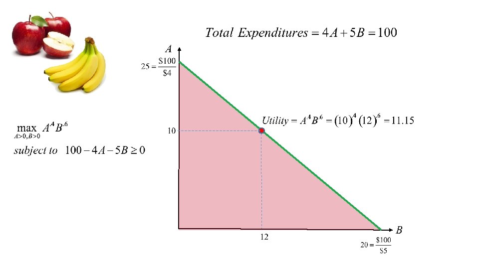
Suppose that you are choosing purchases of apples and bananas. Your total satisfaction as a function of your consumption of apples and bananas can be written as Happiness Weekly Apple Consumption Weekly Banana Consumption Apples cost $4 each and bananas cost $5 each. You want to maximize your satisfaction given that you have $100 to spend

*Note: Technically, there are two additional constraints here But given that zero consumption of either apples or oranges yields zero utility, we can ignore them

Apples cost $4 each and bananas cost $5 each. You want to maximize your satisfaction given that you have $100 to spend So, we set up the lagrangian again Let’s again assume lambda is positive! Take derivatives with respect to ‘A’ and ‘B’ and set the derivatives equal to zero

So we have three equations and three unknowns Lets solve the first two for lambda Set the two expressions for lambda equal to each other and simplify 1 Additional dollar would provide an additional. 11 units of happiness Plug into the last expression and simplify

Non-Binding Constraints

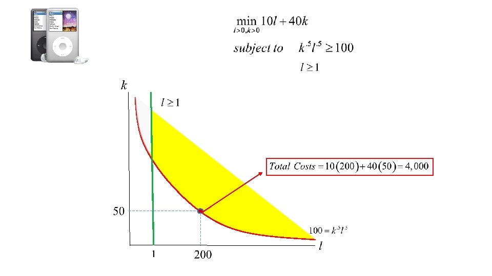
Suppose that you manufacture IPods. Your assembly plant utilizes both labor and capital inputs. You can write your production process as follows Hourly output of IPods Labor inputs Capital Inputs Labor costs $10 per hour and capital costs $40 per unit. Your objective is to minimize the production costs associated with producing 100 IPods per hour. The local government will not allow you to fully automate your plant. That is, you have to use at least 1 hour in your production process

Possible Choices

Minimize the production costs associated with producing 100 IPods per hour while utilizing at least 1 hour of labor. Labor constraint Take derivatives with respect to ‘k’ and ‘l’ and set the derivatives equal to zero Multiplier Conditions

We already know that lambda is positive, but what about the other multiplier? . Suppose that mu is positive as well (i. e. the second constraint is binding) So, we can plug in labor equals 1 Plug in capital equals 10 and solve for lambda and mu This doesn’t work. That means the second constraint is not binding and so we can ignore it

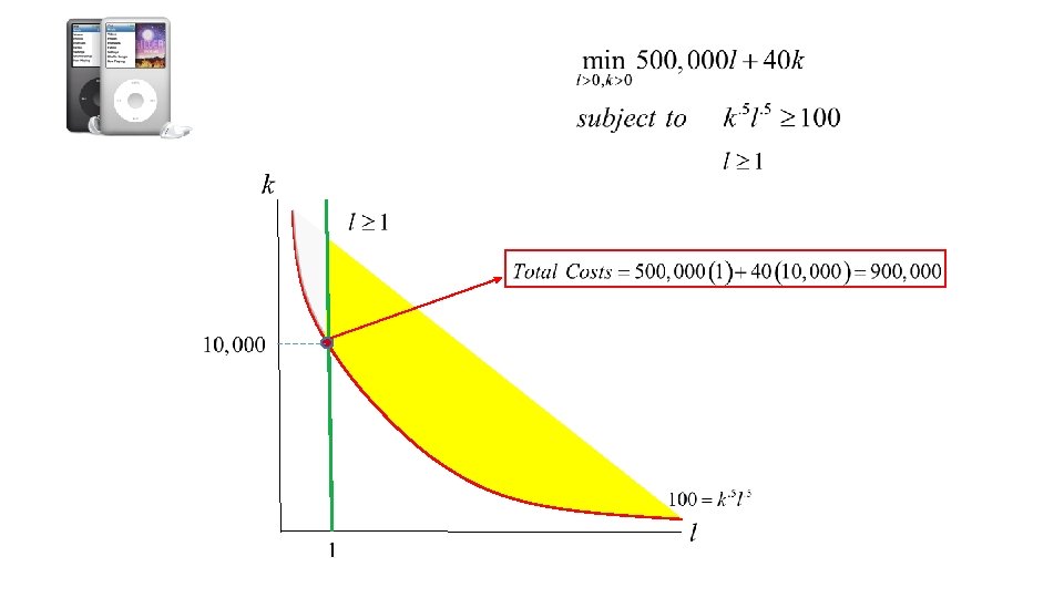
Lets make sure the constraint binds… suppose that labor costs $500, 000 per hour!! Labor constraint Take derivatives with respect to ‘k’ and ‘l’ and set the derivatives equal to zero Multiplier Conditions

We already know that lambda is positive, but what about the other multiplier? . Suppose that mu is positive as well (i. e. the second constraint is binding) So, we can plug in labor equals 1 Plug in capital equals 10 and solve for lambda and mu Now the constraint binds!

So, when does the constraint bind? Lets solve the problem for a generic price of capital, wage, and production requirement Assuming L = 1

Whether or not the constraint binds depends on prices!! Hourly Wage Constraint is Binding Constraint is Non-Binding Price of capital per unit

Let’s go back to the banana/apple problem. However, lets change up the utility function. With the new utility function, we can no longer assume that positive amounts of apples and bananas are consumed!

Write out the lagrangian…. we have three constraints, so we have three multipliers Possible Multiplier Conditions Take derivatives with respect to ‘A’ and ‘B’ and set equal to zero

Possible Multiplier Conditions We can simplify this down a bit. . we already know that the constraint on income will bind Further, consider the change in utility with respect to a change in apple consumption. Zero consumption of apples would make this infinite, so the zero apple constraint will never bind

Now, let’s solve for the conditions under which the zero banana condition binds

Once again, prices determine whether or not the constraint is binding! Constraint is Binding Constraint is Non-Binding