Managerial Economics Estimating Demand Example Aalto University School


 = AP(t)bε(t) which can be presented")
 What substitutes do consumers have for coffee? If tea is")
 for")

 Other data: Average price of a slice of pizza sold on")
 The regression model to be estimated is as follows: Y =")
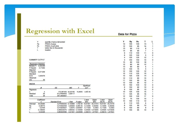
 The estimation result is: Y = 26. 67 – 0. 088*PP")

 How to interpret these results? Are the signs of the estimated")
 How much a one dollar (100 cents) increase in the price")
- Slides: 13
Managerial Economics Estimating Demand Example Aalto University School of Science Department of Industrial Engineering and Management January 10 – 26, 2017 Dr. Arto Kovanen, Ph. D. Visiting Lecturer
General observations Estimating parameters of demand functions can be challenging We cannot observe the utility function/level of utility Utility functions and incomes vary between consumers We only observe the aggregate traded amount, which may be different than demanded by consumers Observed prices are suppose to be equilibrium prices (not always the case) This gives rise to simultaneous equation bias (both P and Q are determined at the same time) and identification problem (is it the demand or supply curve)
Estimating demand A non-linear demand equation for Q(t) = AP(t)bε(t) which can be presented in a linear form as follows Ln. Q(t) = Ln. A + b*ln. P(t) + lnε(t) where b can be interpreted as the price elasticity of demand for Q and ε is the random error term For OLS to be valid, b and P should be uncorrelated with the error term For instance, if Q is demand for coffee and P is the price of coffee
Estimating demand (cont. ) What substitutes do consumers have for coffee? If tea is a substitute for coffee, the demand for coffee will also depend on the price of tea Hence the error term will depend of the price of tea If the prices of coffee and tea are correlated, then the OLS technique will produce a biased estimate of “b” Hence it is important to incorporate variables other than own price and income in the demand estimation
Estimating demand for coffee U. S. coffee demand (Huang, Siegfried and Zardoshty, 1980) for period 1961 – 1977, using quarterly data: ln. Q(t) = 1. 27 – 0. 16*ln. PC(t) + 0. 51*ln. Y(t) (- 2. 14) (1. 23) + 0. 15 ln*PT(t) – 0. 01*Trend(t) – 0. 10*D 1 (0. 55) (-3. 33) – 0. 16*D 2 – 0. 01*D 3 R 2 = 0. 80 where PC = price of coffee, Y = per capita disposal income, PT = price of tea, Q = coffee consumption per head, and Ds are dummy variables
Regression for pizza This is taken from previous course material prepared by Professor Hannele Wallenius Data concerns the consumption of pizza among college students in America What variables are likely to be important for explaining the demand for pizza? What kind of data is collected? Data covers 30 college campuses (for a given period t) Average number of slices of pizza consumed per month
Regression (cont. ) Other data: Average price of a slice of pizza sold on the campus Price of soft drink (complementary product consumed together with pizza; recall that Americans under the age of 21 are not legally allowed to consumer alcoholic drinks) Tuition fee (a proxy for income; higher tuition fee implies higher income (of the parents)) Location of the campus (urban=1, non-urban=0); this is a proxy for substitutes for pizza (i. e. , are the other dinner options, such as Chinese, Mexican, etc. )
Regression (cont. ) The regression model to be estimated is as follows: Y = a + b 1*PP + b 2*PS + b 3*T + b 4*L where a = intercept PP = price of pizza slice (in cents) PS = price of soft drink (in cents) T = tuition (in thousands of US dollars) L = location (dummy variable)
Regression (cont. ) The estimation result is: Y = 26. 67 – 0. 088*PP - 0. 076*PS + 0. 13*T – 0. 544*L (3. 28)* (0. 018)* (0. 020)* (0. 087) (0. 884) R-square = 0. 717 R-square adjusted for degrees of freedom = 0. 67 F – statistic = 15. 8 (significant) Numbers in parenthesis are t-test values
Regression – Chart actual and forecast 16. 00 14. 00 12. 00 10. 00 8. 00 6. 00 4. 00 2. 00 0. 00 1 2 3 4 5 6 7 8 9 10 11 12 13 14 15 16 17 18 19 20 21 22 23 24 25 26 27 28 29 30 Y-hat Y
Regression (cont. ) How to interpret these results? Are the signs of the estimated parameters consistent with theory? What should be the sign of PP (law of demand)? What should be the sign of PS (complementary good)? What determines the sign of the income proxy (normal or inferior good)? How about the location variable (recall that urban=0)?
Regression (cont. ) How much a one dollar (100 cents) increase in the price of pizza is going to change the demand for pizza? Is the demand or pizza elastic or inelastic? What is the price elasticity of pizza demand? What is the cross-price elasticity? Stationarity, constancy of variance, autocorrelation Heteroscedasticity (error variance is not constant)