Ctd Local Linear Models LDA cf PCA FA

Ctd. Local Linear Models, LDA (cf. PCA, FA), Mixed Models: Optimizing, Iterating Peter Fox Data Analytics – ITWS-4600/ITWS-6600/MATP-4450 Group 4 Module 13, April 9, 2018 1

Smoothing/ local … • https: //web. njit. edu/all_topics/Prog_Lang_Do cs/html/library/modreg/html/00 Index. html • http: //cran. r-project. org/doc/contrib/Riccirefcard-regression. pdf 2

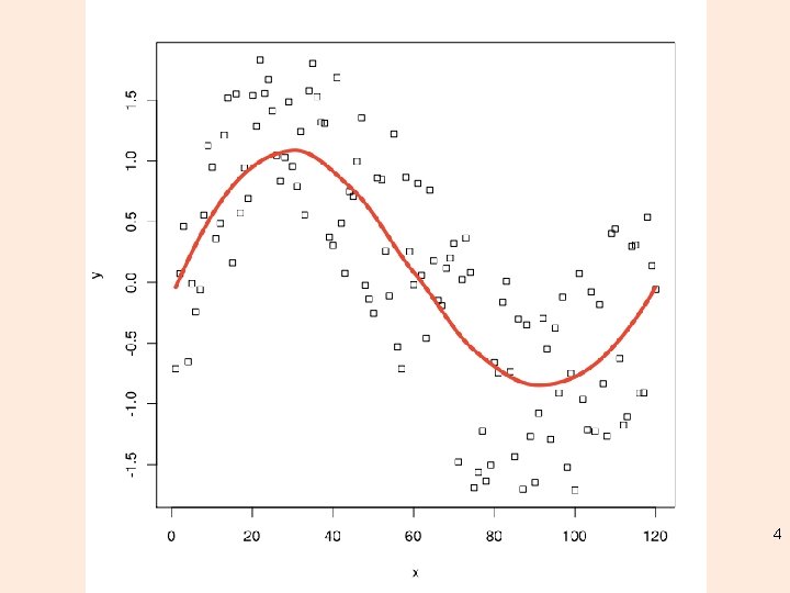
Classes of local regression • Locally (weighted) scatterplot smoothing – LOESS – LOWESS • Fitting is done locally - the fit at point x, the fit is made using points in a neighborhood of x, weighted by their distance from x (with differences in ‘parametric’ variables being ignored when computing the distance) 3

4

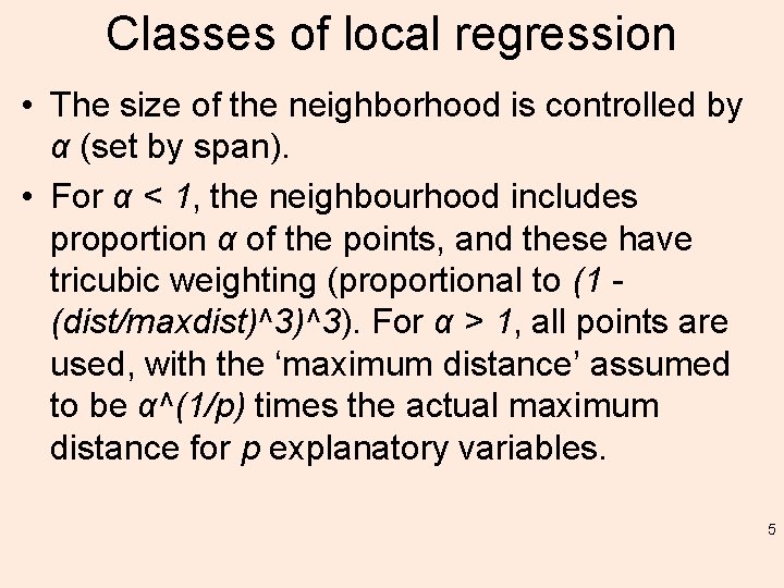
Classes of local regression • The size of the neighborhood is controlled by α (set by span). • For α < 1, the neighbourhood includes proportion α of the points, and these have tricubic weighting (proportional to (1 (dist/maxdist)^3)^3). For α > 1, all points are used, with the ‘maximum distance’ assumed to be α^(1/p) times the actual maximum distance for p explanatory variables. 5

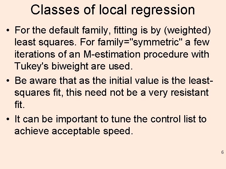
Classes of local regression • For the default family, fitting is by (weighted) least squares. For family="symmetric" a few iterations of an M-estimation procedure with Tukey's biweight are used. • Be aware that as the initial value is the leastsquares fit, this need not be a very resistant fit. • It can be important to tune the control list to achieve acceptable speed. 6

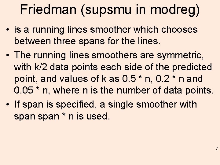
Friedman (supsmu in modreg) • is a running lines smoother which chooses between three spans for the lines. • The running lines smoothers are symmetric, with k/2 data points each side of the predicted point, and values of k as 0. 5 * n, 0. 2 * n and 0. 05 * n, where n is the number of data points. • If span is specified, a single smoother with span * n is used. 7

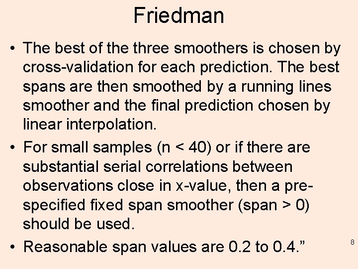
Friedman • The best of the three smoothers is chosen by cross-validation for each prediction. The best spans are then smoothed by a running lines smoother and the final prediction chosen by linear interpolation. • For small samples (n < 40) or if there are substantial serial correlations between observations close in x-value, then a prespecified fixed span smoother (span > 0) should be used. • Reasonable span values are 0. 2 to 0. 4. ” 8

Local non-param • lplm (in Rearrangement) • Local nonparametric method, local linear regression estimator with box kernel (default), for conditional mean functions 9

Ridge regression • Addresses ill-posed regression problems using filtering approaches (e. g. high-pass) • Often called “regularization” • lm. ridge (in MASS) 10

• Quantile regression – is desired if conditional quantile functions are of interest. One advantage of quantile regression, relative to the ordinary least squares regression, is that the quantile regression estimates are more robust against outliers in the response measurements – In practice we often prefer using different measures of central tendency and statistical dispersion to obtain a more comprehensive analysis of the relationship between variables • quantreg (in R) 11

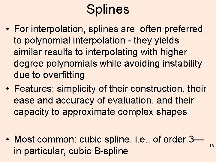
Splines • smooth. spline, splinefun (stats, modreg) and ns (in splines) – http: //www. inside-r. org/r-doc/splines • a numeric function that is piecewise-defined by polynomial functions, and which possesses a sufficiently high degree of smoothness at the places where the polynomial pieces connect (which are known as knots) 12

Splines • For interpolation, splines are often preferred to polynomial interpolation - they yields similar results to interpolating with higher degree polynomials while avoiding instability due to overfitting • Features: simplicity of their construction, their ease and accuracy of evaluation, and their capacity to approximate complex shapes • Most common: cubic spline, i. e. , of order 3— in particular, cubic B-spline 13

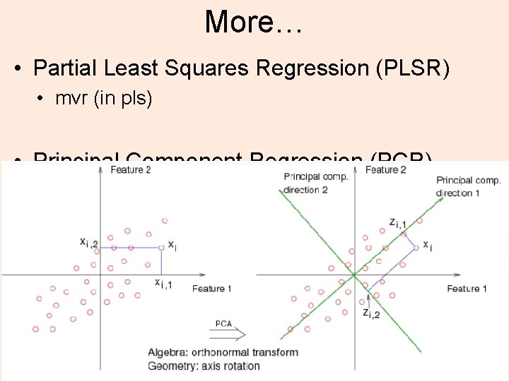
More… • Partial Least Squares Regression (PLSR) • mvr (in pls) • Principal Component Regression (PCR) • Canonical Powered Partial Least Squares (CPPLS) 14

• PCR creates components to explain the observed variability in the predictor variables, without considering the response variable at all • On the other hand, PLSR does take the response variable into account, and therefore often leads to models that are able to fit the response variable with fewer components • Whether or not that ultimately translates into a better model, in terms of its practical use, 15 depends on the context

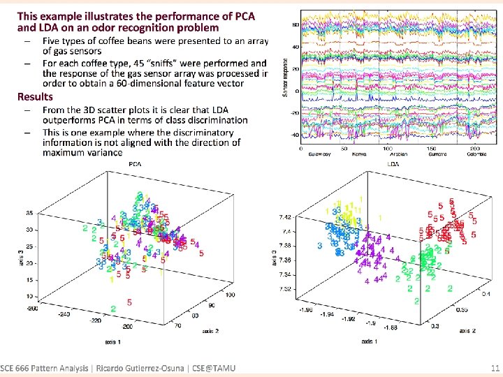
Linear Discriminant Analysis • Find a linear combination of features that characterizes or separates two or more classes of objects or events, i. e. a linear classifier, c. f. dimension reduction then classification (multiple classes, e. g. facial rec. ) • Library lda in package MASS • Dependent variable (the class) is categorial and independent variables are continuous • Assumes normal distribution of classes and equal class co-variances, c. f. Fisher LD does 16 not (fda. CMA in package CMA)

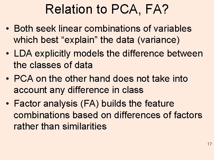
Relation to PCA, FA? • Both seek linear combinations of variables which best “explain” the data (variance) • LDA explicitly models the difference between the classes of data • PCA on the other hand does not take into account any difference in class • Factor analysis (FA) builds the feature combinations based on differences of factors rather than similarities 17

18

Relation to PCA, FA? • Discriminant analysis is not an interdependence technique: a distinction between independent variables and dependent variables is made (cf. different from factor analysis) • NB: If you have categorical independent variables, the equivalent technique is Discriminant Correspondence Analysis (discrimin. coa in ade 4) • See also Flexible DA (fda) and Mixture DA (mda) in mda 19

Now mixed models 20

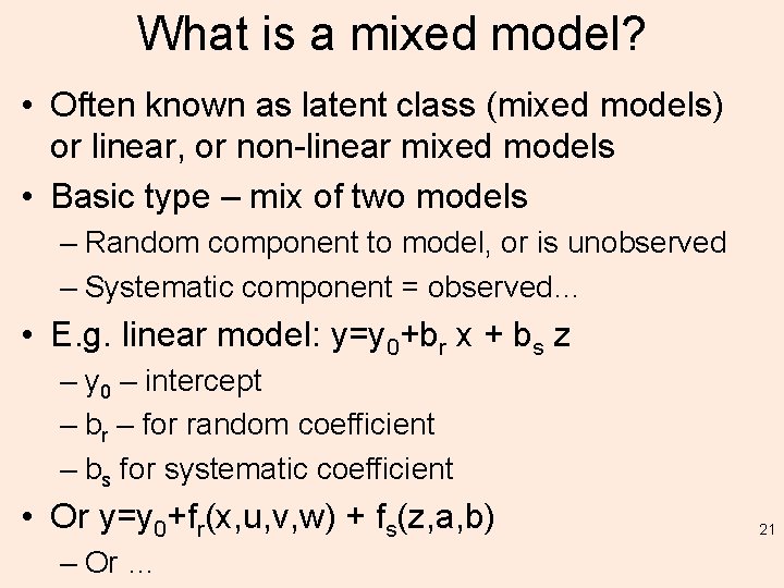
What is a mixed model? • Often known as latent class (mixed models) or linear, or non-linear mixed models • Basic type – mix of two models – Random component to model, or is unobserved – Systematic component = observed… • E. g. linear model: y=y 0+br x + bs z – y 0 – intercept – br – for random coefficient – bs for systematic coefficient • Or y=y 0+fr(x, u, v, w) + fs(z, a, b) – Or … 21

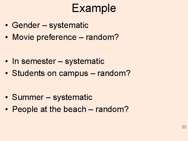
Example • Gender – systematic • Movie preference – random? • In semester – systematic • Students on campus – random? • Summer – systematic • People at the beach – random? 22

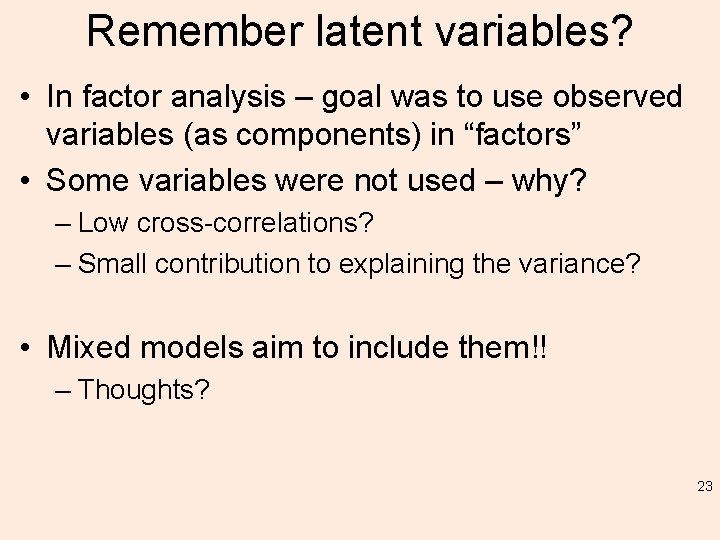
Remember latent variables? • In factor analysis – goal was to use observed variables (as components) in “factors” • Some variables were not used – why? – Low cross-correlations? – Small contribution to explaining the variance? • Mixed models aim to include them!! – Thoughts? 23

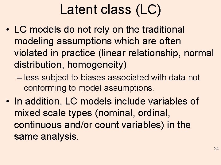
Latent class (LC) • LC models do not rely on the traditional modeling assumptions which are often violated in practice (linear relationship, normal distribution, homogeneity) – less subject to biases associated with data not conforming to model assumptions. • In addition, LC models include variables of mixed scale types (nominal, ordinal, continuous and/or count variables) in the same analysis. 24

Latent class (LC) • For improved cluster or segment description the relationship between the latent classes and external variables (covariates) can be assessed simultaneously with the identification of the clusters. – eliminates the need for the usual second stage of analysis where a discriminant analysis is performed to relate the cluster results to demographic and other variables. 25

Kinds of Latent Class Models • Three common statistical application areas of LC analysis are those that involve – 1) clustering of cases, – 2) variable reduction and scale construction, and – 3) prediction. 26

Thus! • To construct and then run a mixed model, YOU must make many choices including: – the nature of the hierarchy, – the fixed effects and, – the random effects. 27

Beyond mixture = 2? • Hierarchy, fixed, random = 3? • More? • Changes over time – a fourth dimension? 28

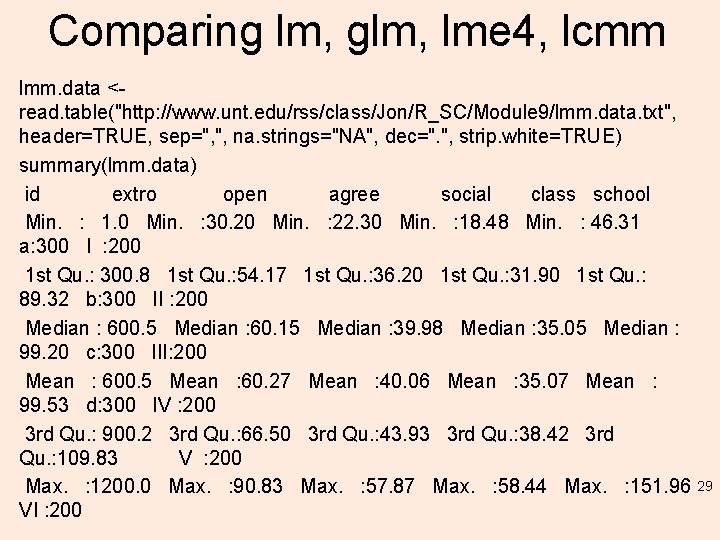
Comparing lm, glm, lme 4, lcmm lmm. data <read. table("http: //www. unt. edu/rss/class/Jon/R_SC/Module 9/lmm. data. txt", header=TRUE, sep=", ", na. strings="NA", dec=". ", strip. white=TRUE) summary(lmm. data) id extro open agree social class school Min. : 1. 0 Min. : 30. 20 Min. : 22. 30 Min. : 18. 48 Min. : 46. 31 a: 300 I : 200 1 st Qu. : 300. 8 1 st Qu. : 54. 17 1 st Qu. : 36. 20 1 st Qu. : 31. 90 1 st Qu. : 89. 32 b: 300 II : 200 Median : 600. 5 Median : 60. 15 Median : 39. 98 Median : 35. 05 Median : 99. 20 c: 300 III: 200 Mean : 600. 5 Mean : 60. 27 Mean : 40. 06 Mean : 35. 07 Mean : 99. 53 d: 300 IV : 200 3 rd Qu. : 900. 2 3 rd Qu. : 66. 50 3 rd Qu. : 43. 93 3 rd Qu. : 38. 42 3 rd Qu. : 109. 83 V : 200 Max. : 1200. 0 Max. : 90. 83 Max. : 57. 87 Max. : 58. 44 Max. : 151. 96 VI : 200 29

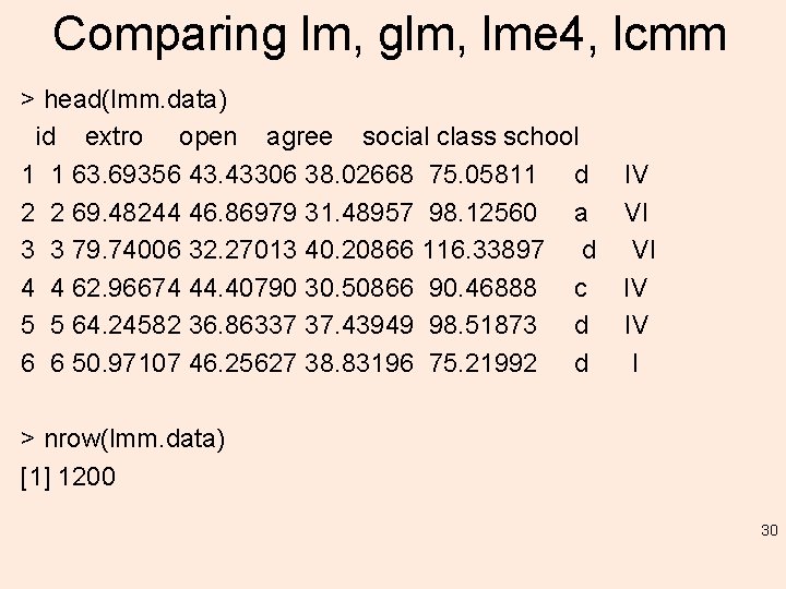
Comparing lm, glm, lme 4, lcmm > head(lmm. data) id extro open agree social class school 1 1 63. 69356 43. 43306 38. 02668 75. 05811 d 2 2 69. 48244 46. 86979 31. 48957 98. 12560 a 3 3 79. 74006 32. 27013 40. 20866 116. 33897 d 4 4 62. 96674 44. 40790 30. 50866 90. 46888 c 5 5 64. 24582 36. 86337 37. 43949 98. 51873 d 6 6 50. 97107 46. 25627 38. 83196 75. 21992 d IV VI VI IV IV I > nrow(lmm. data) [1] 1200 30

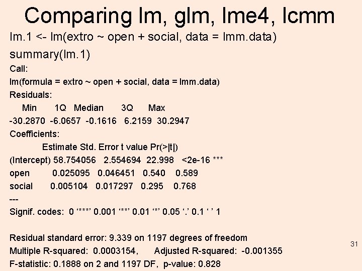
Comparing lm, glm, lme 4, lcmm lm. 1 <- lm(extro ~ open + social, data = lmm. data) summary(lm. 1) Call: lm(formula = extro ~ open + social, data = lmm. data) Residuals: Min 1 Q Median 3 Q Max -30. 2870 -6. 0657 -0. 1616 6. 2159 30. 2947 Coefficients: Estimate Std. Error t value Pr(>|t|) (Intercept) 58. 754056 2. 554694 22. 998 <2 e-16 *** open 0. 025095 0. 046451 0. 540 0. 589 social 0. 005104 0. 017297 0. 295 0. 768 --Signif. codes: 0 ‘***’ 0. 001 ‘**’ 0. 01 ‘*’ 0. 05 ‘. ’ 0. 1 ‘ ’ 1 Residual standard error: 9. 339 on 1197 degrees of freedom Multiple R-squared: 0. 0003154, Adjusted R-squared: -0. 001355 F-statistic: 0. 1888 on 2 and 1197 DF, p-value: 0. 828 31

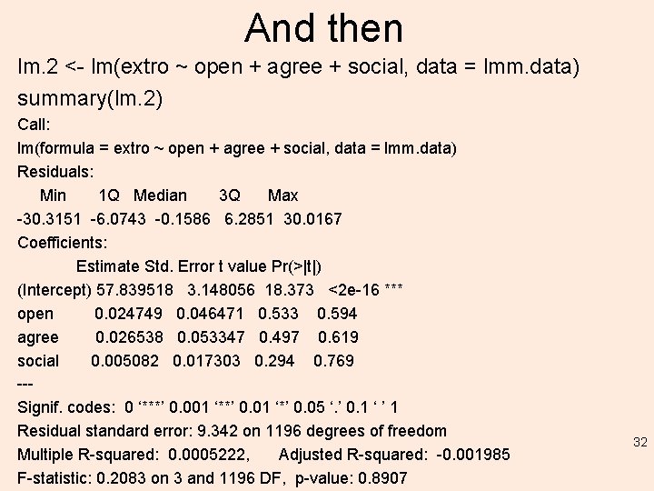
And then lm. 2 <- lm(extro ~ open + agree + social, data = lmm. data) summary(lm. 2) Call: lm(formula = extro ~ open + agree + social, data = lmm. data) Residuals: Min 1 Q Median 3 Q Max -30. 3151 -6. 0743 -0. 1586 6. 2851 30. 0167 Coefficients: Estimate Std. Error t value Pr(>|t|) (Intercept) 57. 839518 3. 148056 18. 373 <2 e-16 *** open 0. 024749 0. 046471 0. 533 0. 594 agree 0. 026538 0. 053347 0. 497 0. 619 social 0. 005082 0. 017303 0. 294 0. 769 --Signif. codes: 0 ‘***’ 0. 001 ‘**’ 0. 01 ‘*’ 0. 05 ‘. ’ 0. 1 ‘ ’ 1 Residual standard error: 9. 342 on 1196 degrees of freedom Multiple R-squared: 0. 0005222, Adjusted R-squared: -0. 001985 F-statistic: 0. 2083 on 3 and 1196 DF, p-value: 0. 8907 32

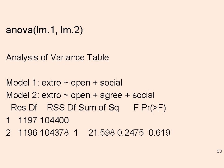
anova(lm. 1, lm. 2) Analysis of Variance Table Model 1: extro ~ open + social Model 2: extro ~ open + agree + social Res. Df RSS Df Sum of Sq F Pr(>F) 1 1197 104400 2 1196 104378 1 21. 598 0. 2475 0. 619 33

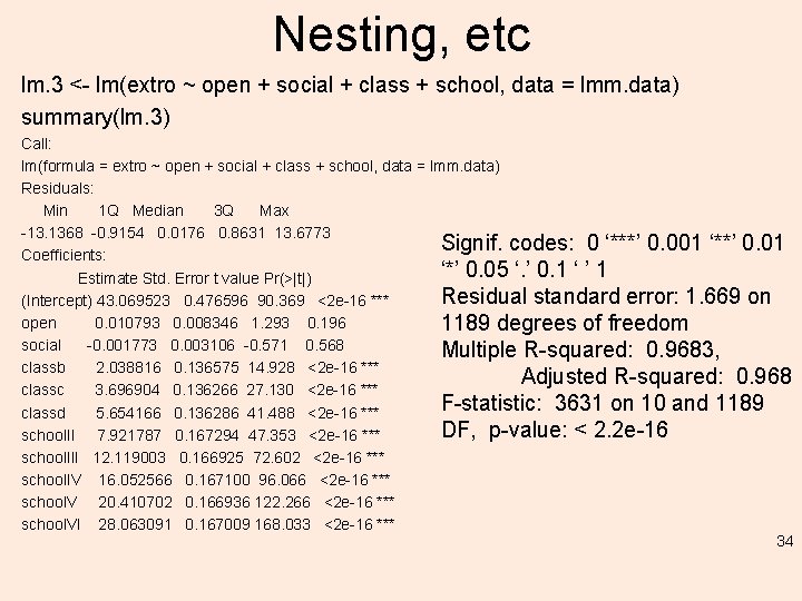
Nesting, etc lm. 3 <- lm(extro ~ open + social + class + school, data = lmm. data) summary(lm. 3) Call: lm(formula = extro ~ open + social + class + school, data = lmm. data) Residuals: Min 1 Q Median 3 Q Max -13. 1368 -0. 9154 0. 0176 0. 8631 13. 6773 Signif. codes: 0 ‘***’ 0. 001 ‘**’ 0. 01 Coefficients: ‘*’ 0. 05 ‘. ’ 0. 1 ‘ ’ 1 Estimate Std. Error t value Pr(>|t|) Residual standard error: 1. 669 on (Intercept) 43. 069523 0. 476596 90. 369 <2 e-16 *** open 0. 010793 0. 008346 1. 293 0. 196 1189 degrees of freedom social -0. 001773 0. 003106 -0. 571 0. 568 Multiple R-squared: 0. 9683, classb 2. 038816 0. 136575 14. 928 <2 e-16 *** Adjusted R-squared: 0. 968 classc 3. 696904 0. 136266 27. 130 <2 e-16 *** F-statistic: 3631 on 10 and 1189 classd 5. 654166 0. 136286 41. 488 <2 e-16 *** DF, p-value: < 2. 2 e-16 school. II 7. 921787 0. 167294 47. 353 <2 e-16 *** school. III 12. 119003 0. 166925 72. 602 <2 e-16 *** school. IV 16. 052566 0. 167100 96. 066 <2 e-16 *** school. V 20. 410702 0. 166936 122. 266 <2 e-16 *** school. VI 28. 063091 0. 167009 168. 033 <2 e-16 *** 34

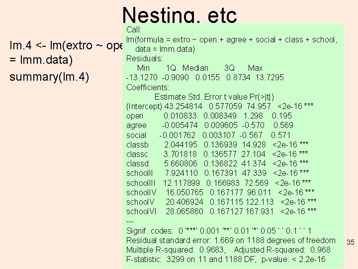
Nesting, etc lm. 4 <- lm(extro ~ = lmm. data) summary(lm. 4) Call: lm(formula = extro ~ open + agree + social + class + school, open data + agree + social + class + school, data = lmm. data) Residuals: Min 1 Q Median 3 Q Max -13. 1270 -0. 9090 0. 0155 0. 8734 13. 7295 Coefficients: Estimate Std. Error t value Pr(>|t|) (Intercept) 43. 254814 0. 577059 74. 957 <2 e-16 *** open 0. 010833 0. 008349 1. 298 0. 195 agree -0. 005474 0. 009605 -0. 570 0. 569 social -0. 001762 0. 003107 -0. 567 0. 571 classb 2. 044195 0. 136939 14. 928 <2 e-16 *** classc 3. 701818 0. 136577 27. 104 <2 e-16 *** classd 5. 660806 0. 136822 41. 374 <2 e-16 *** school. II 7. 924110 0. 167391 47. 339 <2 e-16 *** school. III 12. 117899 0. 166983 72. 569 <2 e-16 *** school. IV 16. 050765 0. 167177 96. 011 <2 e-16 *** school. V 20. 406924 0. 167115 122. 113 <2 e-16 *** school. VI 28. 065860 0. 167127 167. 931 <2 e-16 *** --Signif. codes: 0 ‘***’ 0. 001 ‘**’ 0. 01 ‘*’ 0. 05 ‘. ’ 0. 1 ‘ ’ 1 Residual standard error: 1. 669 on 1188 degrees of freedom 35 Multiple R-squared: 0. 9683, Adjusted R-squared: 0. 968 F-statistic: 3299 on 11 and 1188 DF, p-value: < 2. 2 e-16

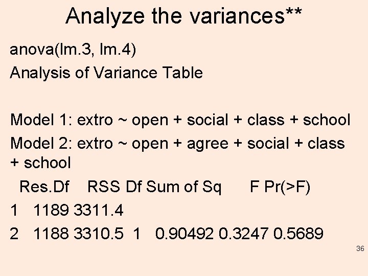
Analyze the variances** anova(lm. 3, lm. 4) Analysis of Variance Table Model 1: extro ~ open + social + class + school Model 2: extro ~ open + agree + social + class + school Res. Df RSS Df Sum of Sq F Pr(>F) 1 1189 3311. 4 2 1188 3310. 5 1 0. 90492 0. 3247 0. 5689 36

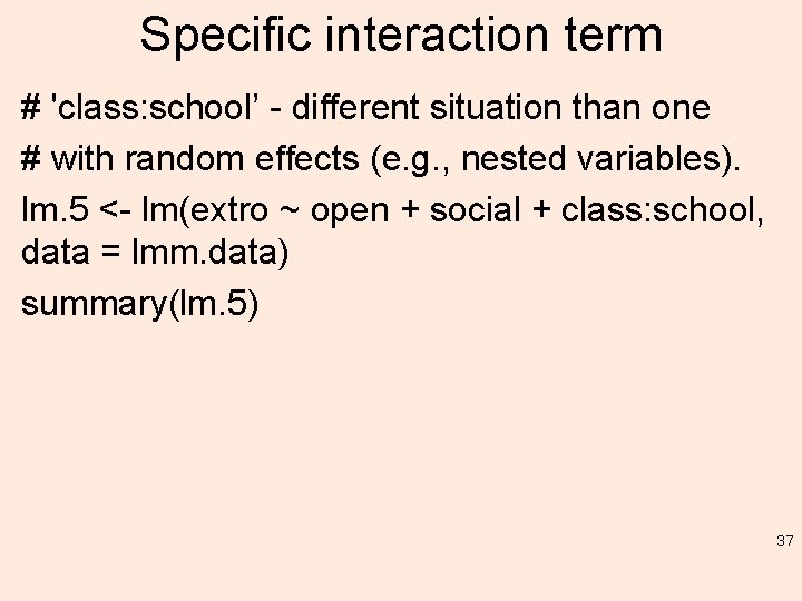
Specific interaction term # 'class: school’ - different situation than one # with random effects (e. g. , nested variables). lm. 5 <- lm(extro ~ open + social + class: school, data = lmm. data) summary(lm. 5) 37

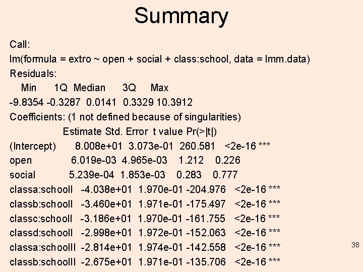
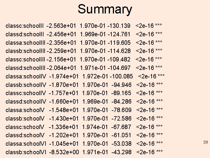
Summary Call: lm(formula = extro ~ open + social + class: school, data = lmm. data) Residuals: Min 1 Q Median 3 Q Max -9. 8354 -0. 3287 0. 0141 0. 3329 10. 3912 Coefficients: (1 not defined because of singularities) Estimate Std. Error t value Pr(>|t|) (Intercept) 8. 008 e+01 3. 073 e-01 260. 581 <2 e-16 *** open 6. 019 e-03 4. 965 e-03 1. 212 0. 226 social 5. 239 e-04 1. 853 e-03 0. 283 0. 777 classa: school. I -4. 038 e+01 1. 970 e-01 -204. 976 <2 e-16 *** classb: school. I -3. 460 e+01 1. 971 e-01 -175. 497 <2 e-16 *** classc: school. I -3. 186 e+01 1. 970 e-01 -161. 755 <2 e-16 *** classd: school. I -2. 998 e+01 1. 972 e-01 -152. 063 <2 e-16 *** classa: school. II -2. 814 e+01 1. 974 e-01 -142. 558 <2 e-16 *** classb: school. II -2. 675 e+01 1. 971 e-01 -135. 706 <2 e-16 *** 38

Summary classc: school. II -2. 563 e+01 1. 970 e-01 -130. 139 classd: school. II -2. 456 e+01 1. 969 e-01 -124. 761 classa: school. III -2. 356 e+01 1. 970 e-01 -119. 605 classb: school. III -2. 259 e+01 1. 970 e-01 -114. 628 classc: school. III -2. 156 e+01 1. 970 e-01 -109. 482 classd: school. III -2. 064 e+01 1. 971 e-01 -104. 697 classa: school. IV -1. 974 e+01 1. 972 e-01 -100. 085 classb: school. IV -1. 870 e+01 1. 970 e-01 -94. 946 classc: school. IV -1. 757 e+01 1. 970 e-01 -89. 165 classd: school. IV -1. 660 e+01 1. 969 e-01 -84. 286 classa: school. V -1. 548 e+01 1. 970 e-01 -78. 609 classb: school. V -1. 430 e+01 1. 970 e-01 -72. 586 classc: school. V -1. 336 e+01 1. 974 e-01 -67. 687 classd: school. V -1. 202 e+01 1. 970 e-01 -61. 051 classa: school. VI -1. 045 e+01 1. 970 e-01 -53. 038 classb: school. VI -8. 532 e+00 1. 971 e-01 -43. 298 <2 e-16 *** <2 e-16 *** <2 e-16 *** <2 e-16 *** 39

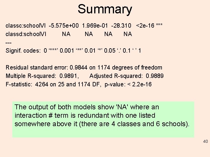
Summary classc: school. VI -5. 575 e+00 1. 969 e-01 -28. 310 <2 e-16 *** classd: school. VI NA NA --Signif. codes: 0 ‘***’ 0. 001 ‘**’ 0. 01 ‘*’ 0. 05 ‘. ’ 0. 1 ‘ ’ 1 Residual standard error: 0. 9844 on 1174 degrees of freedom Multiple R-squared: 0. 9891, Adjusted R-squared: 0. 9889 F-statistic: 4264 on 25 and 1174 DF, p-value: < 2. 2 e-16 The output of both models show 'NA' where an interaction # term is redundant with one listed somewhere above it (there are 4 classes and 6 schools). 40

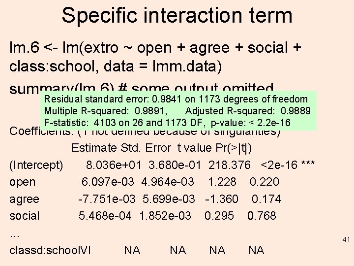
Specific interaction term lm. 6 <- lm(extro ~ open + agree + social + class: school, data = lmm. data) summary(lm. 6) # some output omitted… Residual standard error: 0. 9841 on 1173 degrees of freedom Multiple R-squared: 0. 9891, Adjusted R-squared: 0. 9889 F-statistic: 4103 on 26 and 1173 DF, p-value: < 2. 2 e-16 Coefficients: (1 not defined because of singularities) Estimate Std. Error t value Pr(>|t|) (Intercept) 8. 036 e+01 3. 680 e-01 218. 376 <2 e-16 *** open 6. 097 e-03 4. 964 e-03 1. 228 0. 220 agree -7. 751 e-03 5. 699 e-03 -1. 360 0. 174 social 5. 468 e-04 1. 852 e-03 0. 295 0. 768 … classd: school. VI NA NA 41

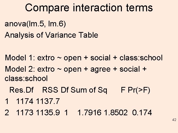
Compare interaction terms anova(lm. 5, lm. 6) Analysis of Variance Table Model 1: extro ~ open + social + class: school Model 2: extro ~ open + agree + social + class: school Res. Df RSS Df Sum of Sq F Pr(>F) 1 1174 1137. 7 2 1173 1135. 9 1 1. 7916 1. 8502 0. 174 42

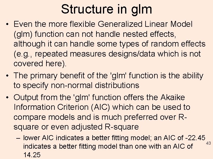
Structure in glm • Even the more flexible Generalized Linear Model (glm) function can not handle nested effects, although it can handle some types of random effects (e. g. , repeated measures designs/data which is not covered here). • The primary benefit of the 'glm' function is the ability to specify non-normal distributions • Output from the 'glm' function offers the Akaike Information Criterion (AIC) which can be used to compare models and is much preferred over Rsquare or even adjusted R-square – lower AIC indicates a better fitting model; an AIC of -22. 45 43 indicates a better fitting model than one with an AIC of 14. 25

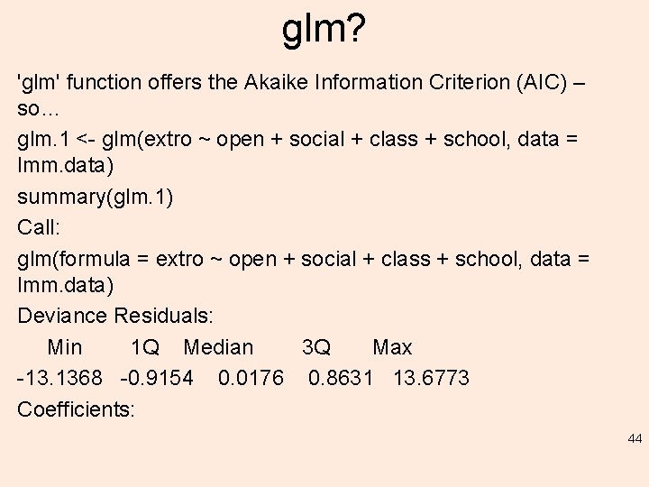
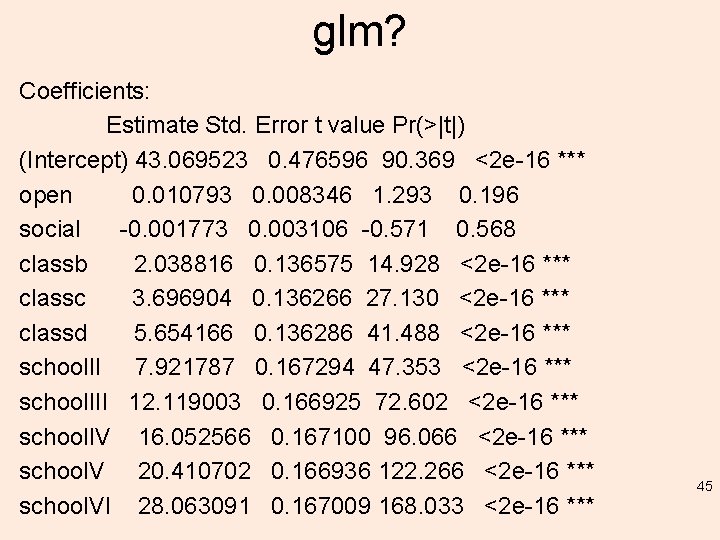
glm? 'glm' function offers the Akaike Information Criterion (AIC) – so… glm. 1 <- glm(extro ~ open + social + class + school, data = lmm. data) summary(glm. 1) Call: glm(formula = extro ~ open + social + class + school, data = lmm. data) Deviance Residuals: Min 1 Q Median 3 Q Max -13. 1368 -0. 9154 0. 0176 0. 8631 13. 6773 Coefficients: 44

glm? Coefficients: Estimate Std. Error t value Pr(>|t|) (Intercept) 43. 069523 0. 476596 90. 369 <2 e-16 *** open 0. 010793 0. 008346 1. 293 0. 196 social -0. 001773 0. 003106 -0. 571 0. 568 classb 2. 038816 0. 136575 14. 928 <2 e-16 *** classc 3. 696904 0. 136266 27. 130 <2 e-16 *** classd 5. 654166 0. 136286 41. 488 <2 e-16 *** school. II 7. 921787 0. 167294 47. 353 <2 e-16 *** school. III 12. 119003 0. 166925 72. 602 <2 e-16 *** school. IV 16. 052566 0. 167100 96. 066 <2 e-16 *** school. V 20. 410702 0. 166936 122. 266 <2 e-16 *** school. VI 28. 063091 0. 167009 168. 033 <2 e-16 *** 45

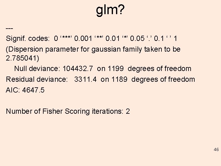
glm? --Signif. codes: 0 ‘***’ 0. 001 ‘**’ 0. 01 ‘*’ 0. 05 ‘. ’ 0. 1 ‘ ’ 1 (Dispersion parameter for gaussian family taken to be 2. 785041) Null deviance: 104432. 7 on 1199 degrees of freedom Residual deviance: 3311. 4 on 1189 degrees of freedom AIC: 4647. 5 Number of Fisher Scoring iterations: 2 46

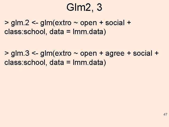
Glm 2, 3 > glm. 2 <- glm(extro ~ open + social + class: school, data = lmm. data) > glm. 3 <- glm(extro ~ open + agree + social + class: school, data = lmm. data) 47

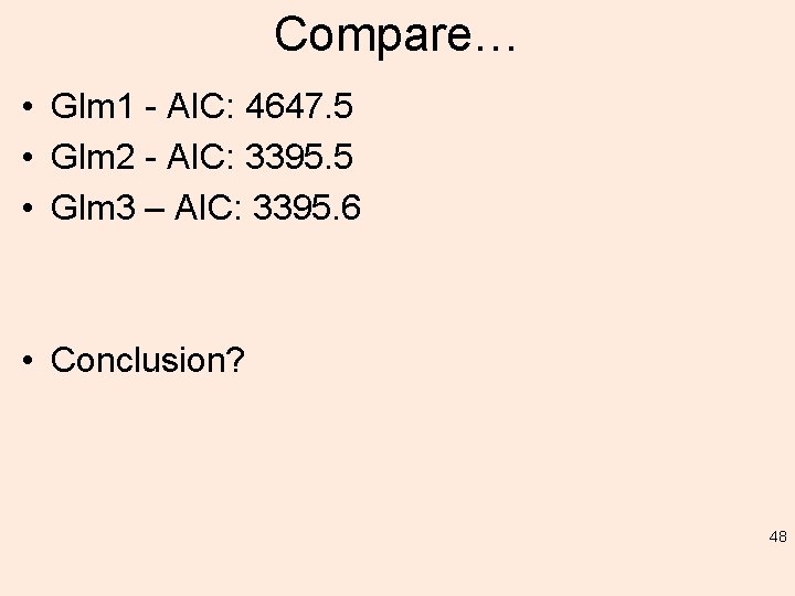
Compare… • Glm 1 - AIC: 4647. 5 • Glm 2 - AIC: 3395. 5 • Glm 3 – AIC: 3395. 6 • Conclusion? 48

However… In order to adequately test these nested (random) effects, we must turn to another type of modeling function/package. > library(lme 4) 49

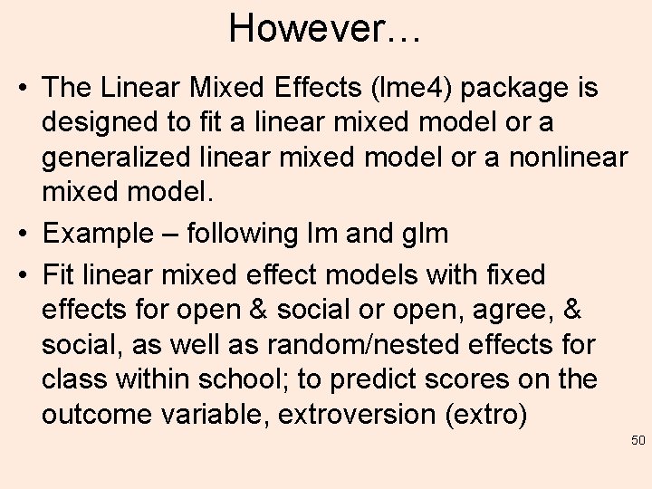
However… • The Linear Mixed Effects (lme 4) package is designed to fit a linear mixed model or a generalized linear mixed model or a nonlinear mixed model. • Example – following lm and glm • Fit linear mixed effect models with fixed effects for open & social or open, agree, & social, as well as random/nested effects for class within school; to predict scores on the outcome variable, extroversion (extro) 50

BIC v. AIC • Note in the output we can use the Baysian Information Criterion (BIC) to compare models; which is similar to, but more conservative than (and thus preferred over) the AIC mentioned previously. • Like AIC; lower BIC reflects better model fit. • 'lmer' function uses REstricted Maximum Likelihood (REML) to estimate the variance components (which is preferred over standard Maximum Likelihood; also available as an 51 option).

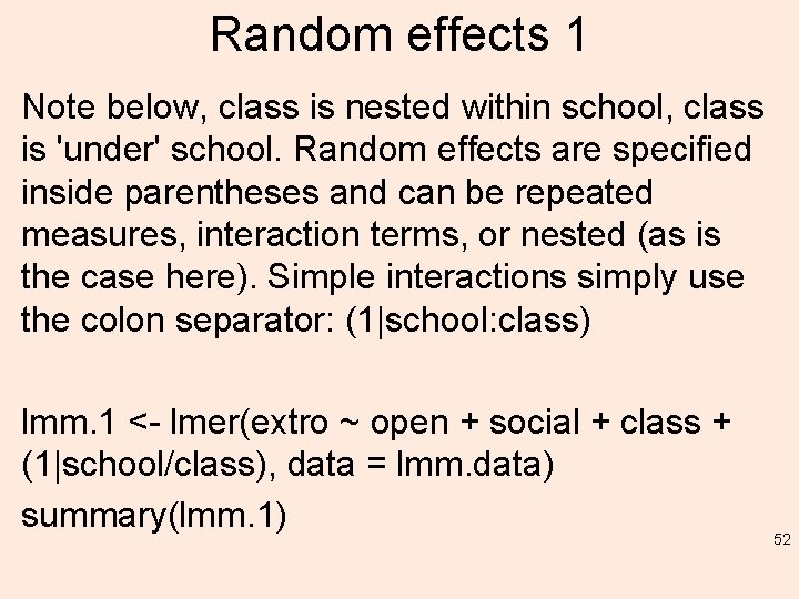
Random effects 1 Note below, class is nested within school, class is 'under' school. Random effects are specified inside parentheses and can be repeated measures, interaction terms, or nested (as is the case here). Simple interactions simply use the colon separator: (1|school: class) lmm. 1 <- lmer(extro ~ open + social + class + (1|school/class), data = lmm. data) summary(lmm. 1) 52

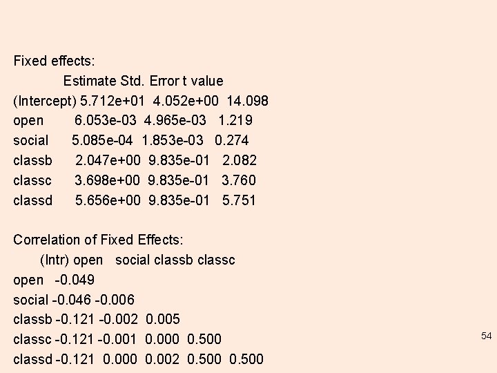
Summary(lmm. 1) Linear mixed model fit by REML ['lmer. Mod'] Formula: extro ~ open + social + class + (1 | school/class) Data: lmm. data REML criterion at convergence: 3521. 5 Scaled residuals: Min 1 Q Median 3 Q Max -10. 0144 -0. 3373 0. 0164 0. 3378 10. 5788 Random effects: Groups Name Variance Std. Dev. class: school (Intercept) 2. 8822 1. 6977 school (Intercept) 95. 1725 9. 7556 Residual 0. 9691 0. 9844 Number of obs: 1200, groups: class: school, 24; school, 6 53

Fixed effects: Estimate Std. Error t value (Intercept) 5. 712 e+01 4. 052 e+00 14. 098 open 6. 053 e-03 4. 965 e-03 1. 219 social 5. 085 e-04 1. 853 e-03 0. 274 classb 2. 047 e+00 9. 835 e-01 2. 082 classc 3. 698 e+00 9. 835 e-01 3. 760 classd 5. 656 e+00 9. 835 e-01 5. 751 Correlation of Fixed Effects: (Intr) open social classb classc open -0. 049 social -0. 046 -0. 006 classb -0. 121 -0. 002 0. 005 classc -0. 121 -0. 001 0. 000 0. 500 classd -0. 121 0. 000 0. 002 0. 500 54

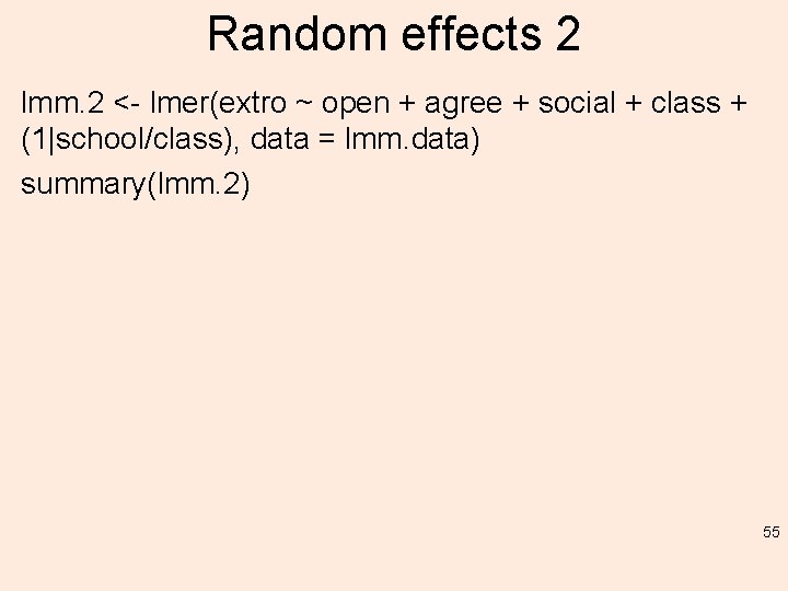
Random effects 2 lmm. 2 <- lmer(extro ~ open + agree + social + class + (1|school/class), data = lmm. data) summary(lmm. 2) 55

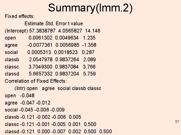
Summary(lmm. 2) Linear mixed model fit by REML ['lmer. Mod'] Formula: extro ~ open + agree + social + class + (1 | school/class) Data: lmm. data REML criterion at convergence: 3528. 1 Scaled residuals: Min 1 Q Median 3 Q Max -10. 0024 -0. 3360 0. 0056 0. 3403 10. 6559 Random effects: Groups Name Variance Std. Dev. class: school (Intercept) 2. 8836 1. 6981 school (Intercept) 95. 1716 9. 7556 Residual 0. 9684 0. 9841 Number of obs: 1200, groups: class: school, 24; school, 6 56

Summary(lmm. 2) Fixed effects: Estimate Std. Error t value (Intercept) 57. 3838787 4. 0565827 14. 146 open 0. 0061302 0. 0049634 1. 235 agree -0. 0077361 0. 0056985 -1. 358 social 0. 0005313 0. 0018523 0. 287 classb 2. 0547978 0. 9837264 2. 089 classc 3. 7049300 0. 9837084 3. 766 classd 5. 6657332 0. 9837204 5. 759 Correlation of Fixed Effects: (Intr) open agree social classb classc open -0. 048 agree -0. 047 -0. 012 social -0. 045 -0. 006 -0. 009 classb -0. 121 -0. 002 -0. 006 0. 005 classc -0. 121 -0. 005 0. 001 0. 500 classd -0. 121 0. 000 -0. 007 0. 002 0. 500 57

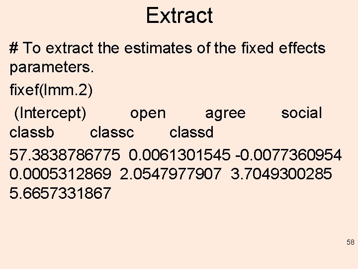
Extract # To extract the estimates of the fixed effects parameters. fixef(lmm. 2) (Intercept) open agree social classb classc classd 57. 3838786775 0. 0061301545 -0. 0077360954 0. 0005312869 2. 0547977907 3. 7049300285 5. 6657331867 58

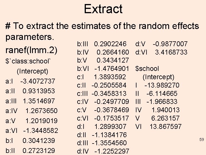
Extract # To extract the estimates of the random effects parameters. b: III 0. 2902246 d: V -0. 9877007 ranef(lmm. 2) b: IV 0. 2664160 d: VI 3. 4168733 $`class: school` (Intercept) a: I -3. 4072737 a: II 0. 9313953 a: III 1. 3514697 a: IV 1. 2673650 a: V 1. 2019019 a: VI -1. 3448582 b: I 0. 3041239 b: II 0. 2723129 b: VI c: II c: IV c: VI d: II d: IV 0. 3434127 -1. 4764901 1. 3893592 -0. 2505584 -0. 3458313 -0. 2497709 -0. 3678469 -0. 1753517 1. 2899307 -1. 1384176 -1. 3554560 -1. 2252297 $school (Intercept) I -13. 989270 II -6. 114665 III -1. 966833 IV 1. 940013 V 6. 263157 VI 13. 867597 59

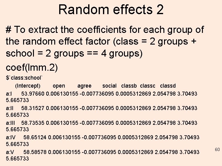
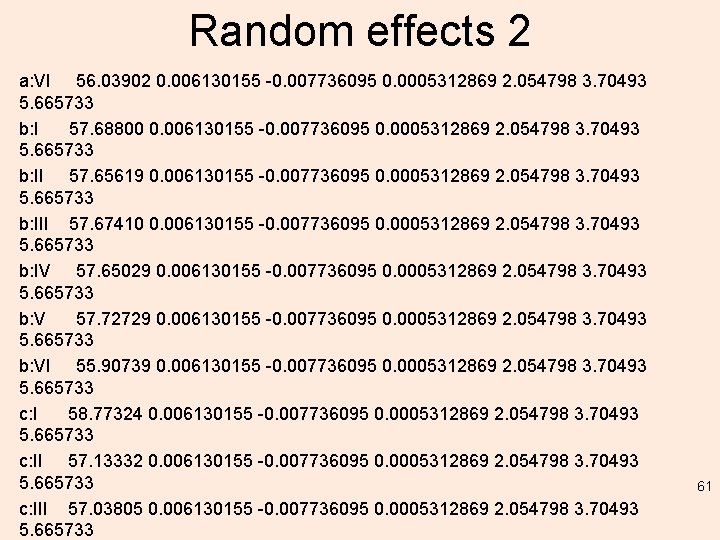
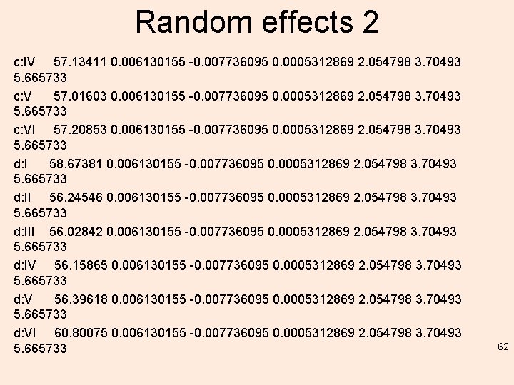
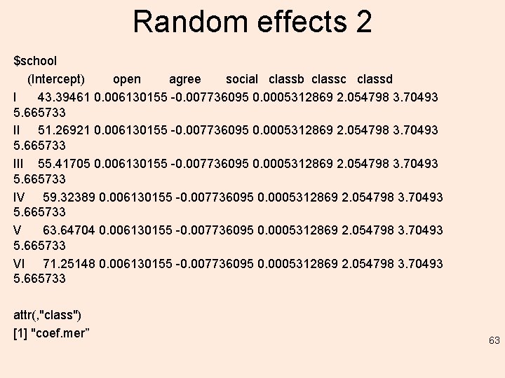
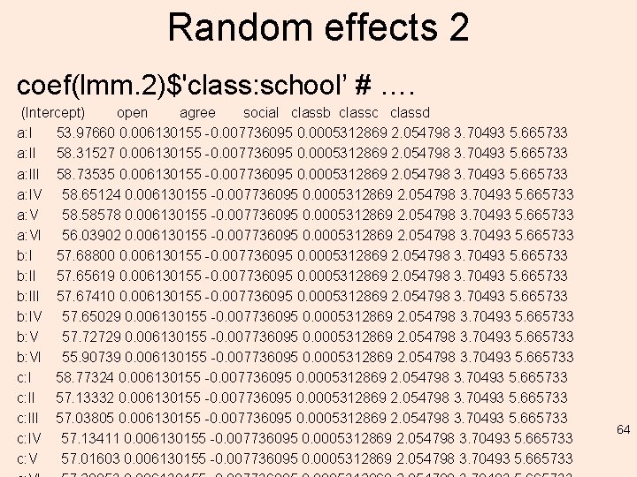
Random effects 2 # To extract the coefficients for each group of the random effect factor (class = 2 groups + school = 2 groups == 4 groups) coef(lmm. 2) $`class: school` (Intercept) open agree social classb classc classd a: I 53. 97660 0. 006130155 -0. 007736095 0. 0005312869 2. 054798 3. 70493 5. 665733 a: II 58. 31527 0. 006130155 -0. 007736095 0. 0005312869 2. 054798 3. 70493 5. 665733 a: III 58. 73535 0. 006130155 -0. 007736095 0. 0005312869 2. 054798 3. 70493 5. 665733 a: IV 58. 65124 0. 006130155 -0. 007736095 0. 0005312869 2. 054798 3. 70493 5. 665733 a: V 58. 58578 0. 006130155 -0. 007736095 0. 0005312869 2. 054798 3. 70493 5. 665733 60

Random effects 2 a: VI 56. 03902 0. 006130155 -0. 007736095 0. 0005312869 2. 054798 3. 70493 5. 665733 b: I 57. 68800 0. 006130155 -0. 007736095 0. 0005312869 2. 054798 3. 70493 5. 665733 b: II 57. 65619 0. 006130155 -0. 007736095 0. 0005312869 2. 054798 3. 70493 5. 665733 b: III 57. 67410 0. 006130155 -0. 007736095 0. 0005312869 2. 054798 3. 70493 5. 665733 b: IV 57. 65029 0. 006130155 -0. 007736095 0. 0005312869 2. 054798 3. 70493 5. 665733 b: V 57. 72729 0. 006130155 -0. 007736095 0. 0005312869 2. 054798 3. 70493 5. 665733 b: VI 55. 90739 0. 006130155 -0. 007736095 0. 0005312869 2. 054798 3. 70493 5. 665733 c: I 58. 77324 0. 006130155 -0. 007736095 0. 0005312869 2. 054798 3. 70493 5. 665733 c: II 57. 13332 0. 006130155 -0. 007736095 0. 0005312869 2. 054798 3. 70493 5. 665733 c: III 57. 03805 0. 006130155 -0. 007736095 0. 0005312869 2. 054798 3. 70493 5. 665733 61

Random effects 2 c: IV 57. 13411 0. 006130155 -0. 007736095 0. 0005312869 2. 054798 3. 70493 5. 665733 c: V 57. 01603 0. 006130155 -0. 007736095 0. 0005312869 2. 054798 3. 70493 5. 665733 c: VI 57. 20853 0. 006130155 -0. 007736095 0. 0005312869 2. 054798 3. 70493 5. 665733 d: I 58. 67381 0. 006130155 -0. 007736095 0. 0005312869 2. 054798 3. 70493 5. 665733 d: II 56. 24546 0. 006130155 -0. 007736095 0. 0005312869 2. 054798 3. 70493 5. 665733 d: III 56. 02842 0. 006130155 -0. 007736095 0. 0005312869 2. 054798 3. 70493 5. 665733 d: IV 56. 15865 0. 006130155 -0. 007736095 0. 0005312869 2. 054798 3. 70493 5. 665733 d: V 56. 39618 0. 006130155 -0. 007736095 0. 0005312869 2. 054798 3. 70493 5. 665733 d: VI 60. 80075 0. 006130155 -0. 007736095 0. 0005312869 2. 054798 3. 70493 5. 665733 62

Random effects 2 $school (Intercept) open agree social classb classc classd I 43. 39461 0. 006130155 -0. 007736095 0. 0005312869 2. 054798 3. 70493 5. 665733 II 51. 26921 0. 006130155 -0. 007736095 0. 0005312869 2. 054798 3. 70493 5. 665733 III 55. 41705 0. 006130155 -0. 007736095 0. 0005312869 2. 054798 3. 70493 5. 665733 IV 59. 32389 0. 006130155 -0. 007736095 0. 0005312869 2. 054798 3. 70493 5. 665733 V 63. 64704 0. 006130155 -0. 007736095 0. 0005312869 2. 054798 3. 70493 5. 665733 VI 71. 25148 0. 006130155 -0. 007736095 0. 0005312869 2. 054798 3. 70493 5. 665733 attr(, "class") [1] "coef. mer” 63

Random effects 2 coef(lmm. 2)$'class: school’ # …. (Intercept) open agree social classb classc classd a: I 53. 97660 0. 006130155 -0. 007736095 0. 0005312869 2. 054798 3. 70493 5. 665733 a: II 58. 31527 0. 006130155 -0. 007736095 0. 0005312869 2. 054798 3. 70493 5. 665733 a: III 58. 73535 0. 006130155 -0. 007736095 0. 0005312869 2. 054798 3. 70493 5. 665733 a: IV 58. 65124 0. 006130155 -0. 007736095 0. 0005312869 2. 054798 3. 70493 5. 665733 a: V 58. 58578 0. 006130155 -0. 007736095 0. 0005312869 2. 054798 3. 70493 5. 665733 a: VI 56. 03902 0. 006130155 -0. 007736095 0. 0005312869 2. 054798 3. 70493 5. 665733 b: I 57. 68800 0. 006130155 -0. 007736095 0. 0005312869 2. 054798 3. 70493 5. 665733 b: II 57. 65619 0. 006130155 -0. 007736095 0. 0005312869 2. 054798 3. 70493 5. 665733 b: III 57. 67410 0. 006130155 -0. 007736095 0. 0005312869 2. 054798 3. 70493 5. 665733 b: IV 57. 65029 0. 006130155 -0. 007736095 0. 0005312869 2. 054798 3. 70493 5. 665733 b: V 57. 72729 0. 006130155 -0. 007736095 0. 0005312869 2. 054798 3. 70493 5. 665733 b: VI 55. 90739 0. 006130155 -0. 007736095 0. 0005312869 2. 054798 3. 70493 5. 665733 c: I 58. 77324 0. 006130155 -0. 007736095 0. 0005312869 2. 054798 3. 70493 5. 665733 c: II 57. 13332 0. 006130155 -0. 007736095 0. 0005312869 2. 054798 3. 70493 5. 665733 c: III 57. 03805 0. 006130155 -0. 007736095 0. 0005312869 2. 054798 3. 70493 5. 665733 c: IV 57. 13411 0. 006130155 -0. 007736095 0. 0005312869 2. 054798 3. 70493 5. 665733 c: V 57. 01603 0. 006130155 -0. 007736095 0. 0005312869 2. 054798 3. 70493 5. 665733 64

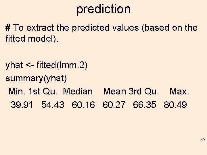
prediction # To extract the predicted values (based on the fitted model). yhat <- fitted(lmm. 2) summary(yhat) Min. 1 st Qu. Median Mean 3 rd Qu. Max. 39. 91 54. 43 60. 16 60. 27 66. 35 80. 49 65

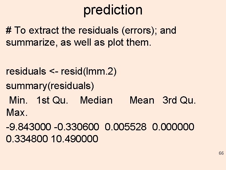
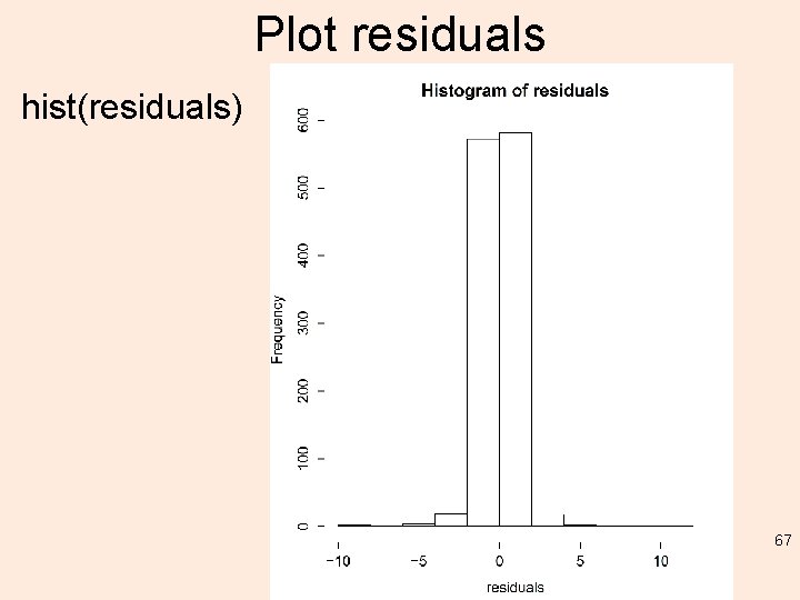
prediction # To extract the residuals (errors); and summarize, as well as plot them. residuals <- resid(lmm. 2) summary(residuals) Min. 1 st Qu. Median Mean 3 rd Qu. Max. -9. 843000 -0. 330600 0. 005528 0. 000000 0. 334800 10. 490000 66

Plot residuals hist(residuals) 67

Reading, etc. • http: //data-informed. com/focus-predictiveanalytics/ • Lab this week • NB. Not covering logistic regression since most students know it – if not: https: //www. rbloggers. com/how-to-perform-a-logisticregression-in-r/ 68