PCA Lecture 2 Recap of PCA what it

PCA: Lecture 2 • Recap of PCA: what it does, how to do it • Details of PCA • presentation of results • terminology • scaling • truncation of PCs • interpretation of PCs • Rotation of PCs • Singular Value Decomposition (SVD) • Applications • Exploratory data analysis (EDA) • Data compression • PC regression / statistical prediction • etc… • Extensions to PCA and Some of its Relatives • Extended EOF (EEOF), Singular spectrum analysis (SSA), Canonical Correlation Analysis (CCA), Principal Oscillation Patterns (POP), Independent Component Analysis (ISA)

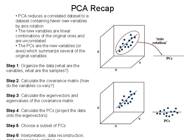
PCA Recap • PCA reduces a correlated dataset to a dataset containing fewer new variables by axis rotation • The new variables are linear combinations of the original ones and are uncorrelated • The PCs are the new variables (or axes) which summarize several of the original variables Step 1: Organize the data (what are the variables, what are the samples? ) Step 2: Calculate the covariance matrix (how do the variables co-vary? ) Step 3: Calculate the eigenvectors and eigenvalues of the covariance matrix Step 4: Calculate the PCs (project the data onto the eigenvectors) Step 5: Choose a subset of PCs Step 6: Interpretation, data reconstruction,

Presentation of PCA Results PCA results in; • a set of eigenvectors which are ordered according to the amount of variance of the original dataset that they explain • the dataset projected onto the PCs (for time series data these are the PC time series) • normally we are only concerned with the top few PCs

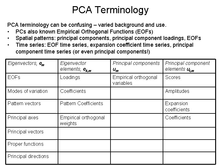
PCA Terminology PCA terminology can be confusing – varied background and use. • PCs also known Empirical Orthogonal Functions (EOFs) • Spatial patterns: principal components, principal component loadings, EOFs • Time series: EOF time series, expansion coefficient time series, principal component time series (or even principal components!) Eigenvectors, em Eigenvector elements, ek, m Principal components um Principal component elements ui, m EOFs Loadings Empirical orthogonal variables Scores Modes of variation Coefficients Amplitudes Pattern vectors Pattern Coefficients Expansion coefficients Principal axes Empirical orthogonal weights Coefficients Principal vectors Proper functions Principal directions

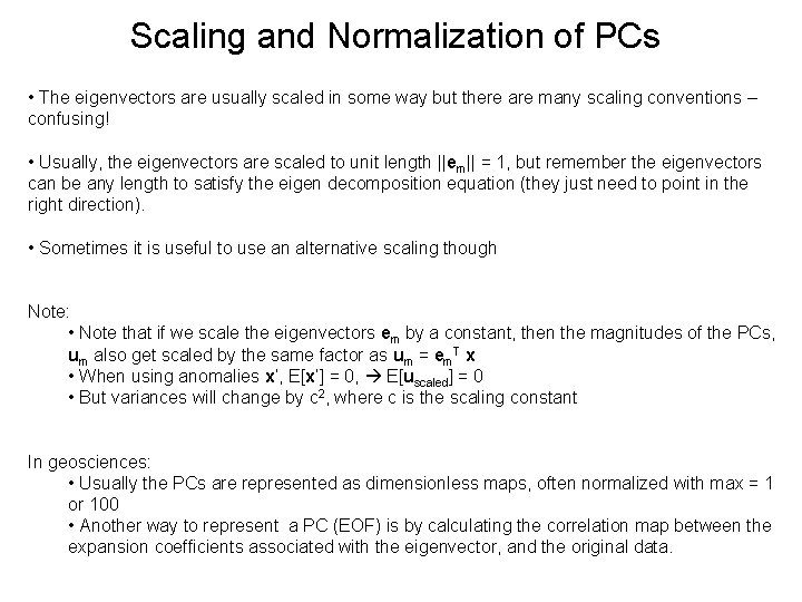
Scaling and Normalization of PCs • The eigenvectors are usually scaled in some way but there are many scaling conventions – confusing! • Usually, the eigenvectors are scaled to unit length ||em|| = 1, but remember the eigenvectors can be any length to satisfy the eigen decomposition equation (they just need to point in the right direction). • Sometimes it is useful to use an alternative scaling though Note: • Note that if we scale the eigenvectors em by a constant, then the magnitudes of the PCs, um also get scaled by the same factor as um = em. T x • When using anomalies x’, E[x’] = 0, E[uscaled] = 0 • But variances will change by c 2, where c is the scaling constant In geosciences: • Usually the PCs are represented as dimensionless maps, often normalized with max = 1 or 100 • Another way to represent a PC (EOF) is by calculating the correlation map between the expansion coefficients associated with the eigenvector, and the original data.

Scaling and Normalization of PCs Some common scalings and their impacts: Eigenvector scaling E[um] Var[um] Corr[um, xk] Corr[um, zk] ||em|| = 1 0 λm ek, m(λm)1/2 / sk ek, m(λ)1/2 ||em|| = (λ)1/2 0 λm 2 ek, m/sk ek, m ||em|| = (λ)-1/2 0 1 ek, m λm/sk ek, m λm Eigenvector elements are more interpretable in terms of the relationship between the PCs and the original data. Each eigenvector element ek, m = correlation ru, z between the mth PC um and the kth standardized variable zk. All PCs have equal unit variance, which can be useful in the detection of outliers

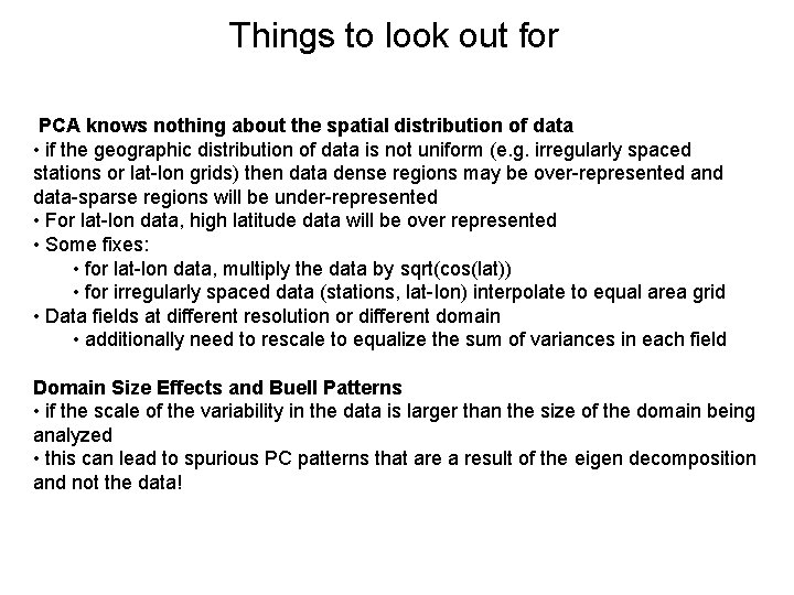
Things to look out for PCA knows nothing about the spatial distribution of data • if the geographic distribution of data is not uniform (e. g. irregularly spaced stations or lat-lon grids) then data dense regions may be over-represented and data-sparse regions will be under-represented • For lat-lon data, high latitude data will be over represented • Some fixes: • for lat-lon data, multiply the data by sqrt(cos(lat)) • for irregularly spaced data (stations, lat-lon) interpolate to equal area grid • Data fields at different resolution or different domain • additionally need to rescale to equalize the sum of variances in each field Domain Size Effects and Buell Patterns • if the scale of the variability in the data is larger than the size of the domain being analyzed • this can lead to spurious PC patterns that are a result of the eigen decomposition and not the data!

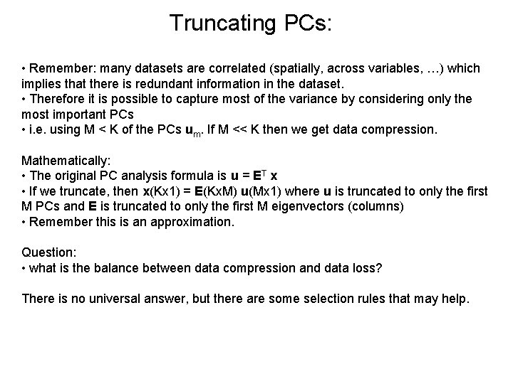
Truncating PCs: • Remember: many datasets are correlated (spatially, across variables, …) which implies that there is redundant information in the dataset. • Therefore it is possible to capture most of the variance by considering only the most important PCs • i. e. using M < K of the PCs um. If M << K then we get data compression. Mathematically: • The original PC analysis formula is u = ET x • If we truncate, then x(Kx 1) = E(Kx. M) u(Mx 1) where u is truncated to only the first M PCs and E is truncated to only the first M eigenvectors (columns) • Remember this is an approximation. Question: • what is the balance between data compression and data loss? There is no universal answer, but there are some selection rules that may help.

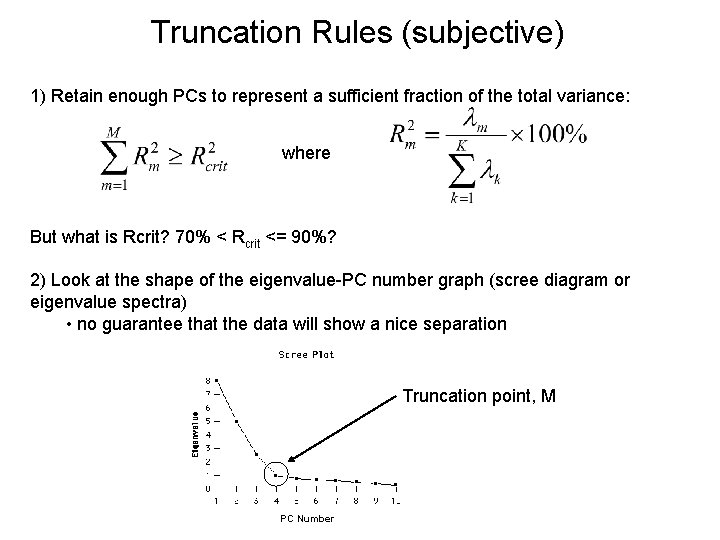
Truncation Rules (subjective) 1) Retain enough PCs to represent a sufficient fraction of the total variance: where But what is Rcrit? 70% < Rcrit <= 90%? 2) Look at the shape of the eigenvalue-PC number graph (scree diagram or eigenvalue spectra) • no guarantee that the data will show a nice separation Truncation point, M PC Number

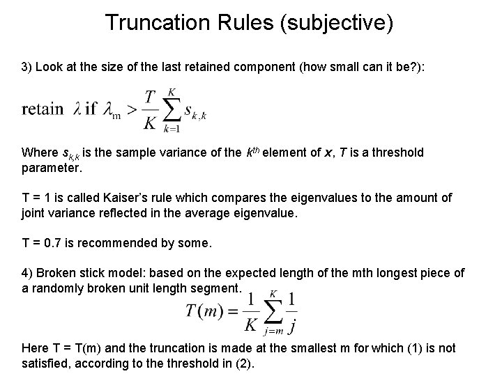
Truncation Rules (subjective) 3) Look at the size of the last retained component (how small can it be? ): Where sk, k is the sample variance of the kth element of x, T is a threshold parameter. T = 1 is called Kaiser’s rule which compares the eigenvalues to the amount of joint variance reflected in the average eigenvalue. T = 0. 7 is recommended by some. 4) Broken stick model: based on the expected length of the mth longest piece of a randomly broken unit length segment. Here T = T(m) and the truncation is made at the smallest m for which (1) is not satisfied, according to the threshold in (2).

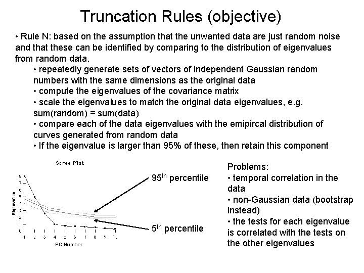
Truncation Rules (objective) • Rule N: based on the assumption that the unwanted data are just random noise and that these can be identified by comparing to the distribution of eigenvalues from random data. • repeatedly generate sets of vectors of independent Gaussian random numbers with the same dimensions as the original data • compute the eigenvalues of the covariance matrix • scale the eigenvalues to match the original data eigenvalues, e. g. sum(random) = sum(data) • compare each of the data eigenvalues with the emipircal distribution of curves generated from random data • If the eigenvalue is larger than 95% of these, then retain this component 95 th percentile PC Number Problems: • temporal correlation in the data • non-Gaussian data (bootstrap instead) • the tests for each eigenvalue is correlated with the tests on the other eigenvalues

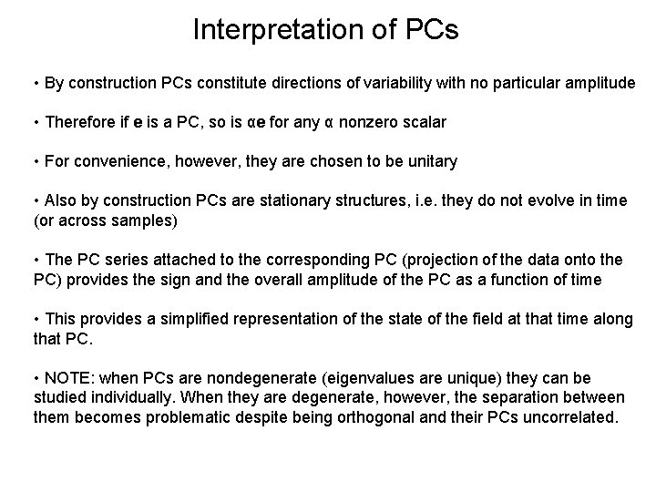
Interpretation of PCs • By construction PCs constitute directions of variability with no particular amplitude • Therefore if e is a PC, so is αe for any α nonzero scalar • For convenience, however, they are chosen to be unitary • Also by construction PCs are stationary structures, i. e. they do not evolve in time (or across samples) • The PC series attached to the corresponding PC (projection of the data onto the PC) provides the sign and the overall amplitude of the PC as a function of time • This provides a simplified representation of the state of the field at that time along that PC. • NOTE: when PCs are nondegenerate (eigenvalues are unique) they can be studied individually. When they are degenerate, however, the separation between them becomes problematic despite being orthogonal and their PCs uncorrelated.

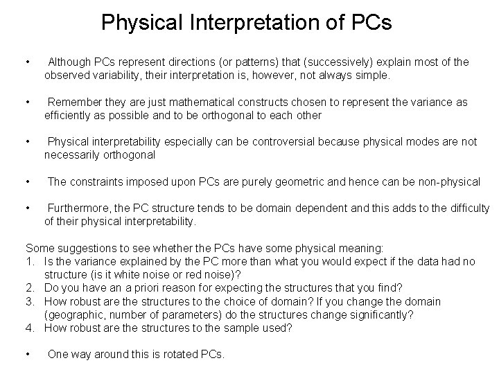
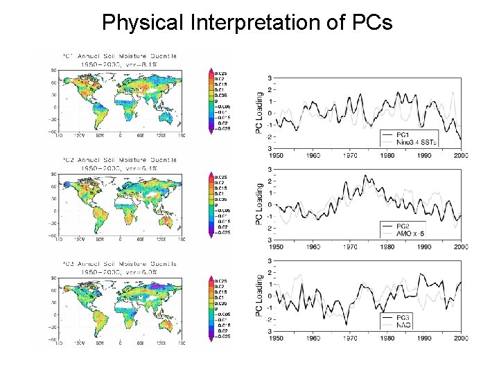
Physical Interpretation of PCs • Although PCs represent directions (or patterns) that (successively) explain most of the observed variability, their interpretation is, however, not always simple. • Remember they are just mathematical constructs chosen to represent the variance as efficiently as possible and to be orthogonal to each other • Physical interpretability especially can be controversial because physical modes are not necessarily orthogonal • The constraints imposed upon PCs are purely geometric and hence can be non-physical • Furthermore, the PC structure tends to be domain dependent and this adds to the difficulty of their physical interpretability. Some suggestions to see whether the PCs have some physical meaning: 1. Is the variance explained by the PC more than what you would expect if the data had no structure (is it white noise or red noise)? 2. Do you have an a priori reason for expecting the structures that you find? 3. How robust are the structures to the choice of domain? If you change the domain (geographic, number of parameters) do the structures change significantly? 4. How robust are the structures to the sample used? • One way around this is rotated PCs.

Physical Interpretation of PCs

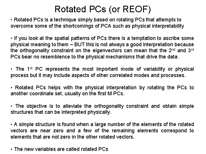
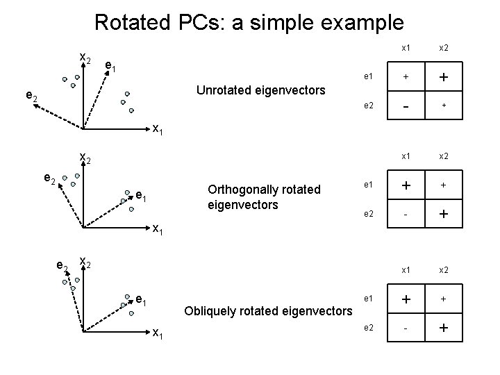
Rotated PCs (or REOF) • Rotated PCs is a technique simply based on rotating PCs that attempts to overcome some of the shortcomings of PCA such as physical interpretability • If you look at the spatial patterns of PCs there is a temptation to ascribe some physical meaning to them – BUT this is not always a good interpretation because the orthogonality constraint on the eigenvectors can mean that the 2 nd and 3 rd PCs bear no resemblence to the physical mechanisms that drive the data. • The 1 st PC represents the most important mode of variability or physical process but it may include aspects of other correlated modes and processes. • Rotated PCs helps with the physical interpretation by rotating the PCs to another coordinate set, usually on the first M PCs. • The objective is to alleviate the orthogonality constraint and obtain simple structures that can be interpreted physically. • A simple structure is found when a large number of the elements of the rotated vectors are near zero and a few of the remaining elements correspond to elements that are not zero in the other rotated vectors. • The new variables are called rotated PCs

Rotated PCs: a simple example x 2 e 1 + + e 2 - + x 1 x 2 e 1 + + e 2 - + Unrotated eigenvectors e 2 x 1 x 2 e 2 Orthogonally rotated eigenvectors e 1 x 1 e 2 x 2 e 1 Obliquely rotated eigenvectors x 1

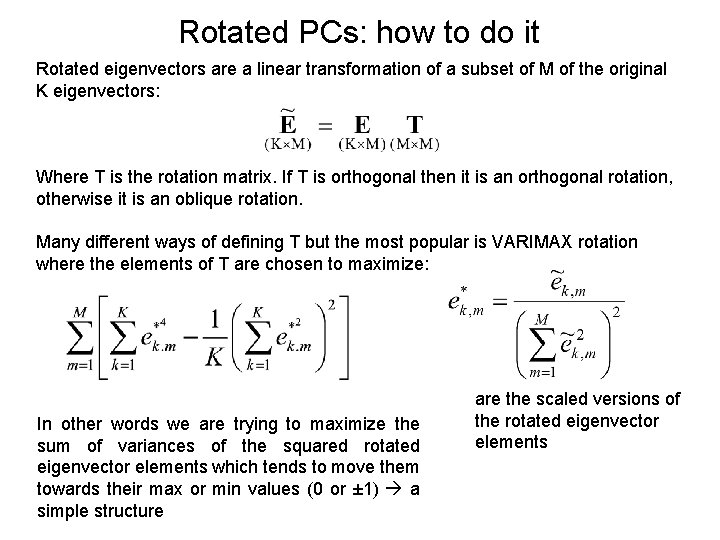
Rotated PCs: how to do it Rotated eigenvectors are a linear transformation of a subset of M of the original K eigenvectors: Where T is the rotation matrix. If T is orthogonal then it is an orthogonal rotation, otherwise it is an oblique rotation. Many different ways of defining T but the most popular is VARIMAX rotation where the elements of T are chosen to maximize: In other words we are trying to maximize the sum of variances of the squared rotated eigenvector elements which tends to move them towards their max or min values (0 or ± 1) a simple structure are the scaled versions of the rotated eigenvector elements

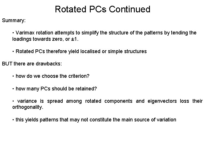
Rotated PCs Continued Summary: • Varimax rotation attempts to simplify the structure of the patterns by tending the loadings towards zero, or ± 1. • Rotated PCs therefore yield localised or simple structures BUT there are drawbacks: • how do we choose the criterion? • how many PCs should be retained? • variance is spread among rotated components and eigenvectors loss their orthogonality. • this yields patterns that may not constitute the main source of variation

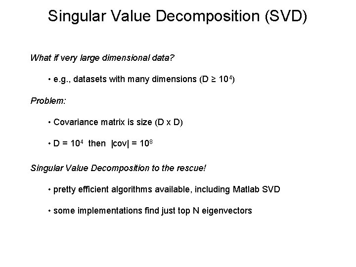
Singular Value Decomposition (SVD) What if very large dimensional data? • e. g. , datasets with many dimensions (D ≥ 104) Problem: • Covariance matrix is size (D x D) • D = 104 then |cov| = 108 Singular Value Decomposition to the rescue! • pretty efficient algorithms available, including Matlab SVD • some implementations find just top N eigenvectors

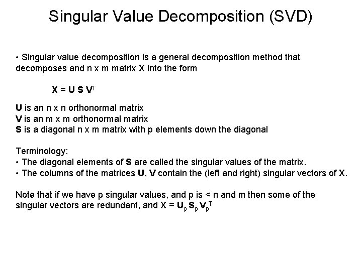
Singular Value Decomposition (SVD) • Singular value decomposition is a general decomposition method that decomposes and n x m matrix X into the form X = U S VT U is an n x n orthonormal matrix V is an m x m orthonormal matrix S is a diagonal n x m matrix with p elements down the diagonal Terminology: • The diagonal elements of S are called the singular values of the matrix. • The columns of the matrices U, V contain the (left and right) singular vectors of X. Note that if we have p singular values, and p is < n and m then some of the singular vectors are redundant, and X = Up Sp Vp. T

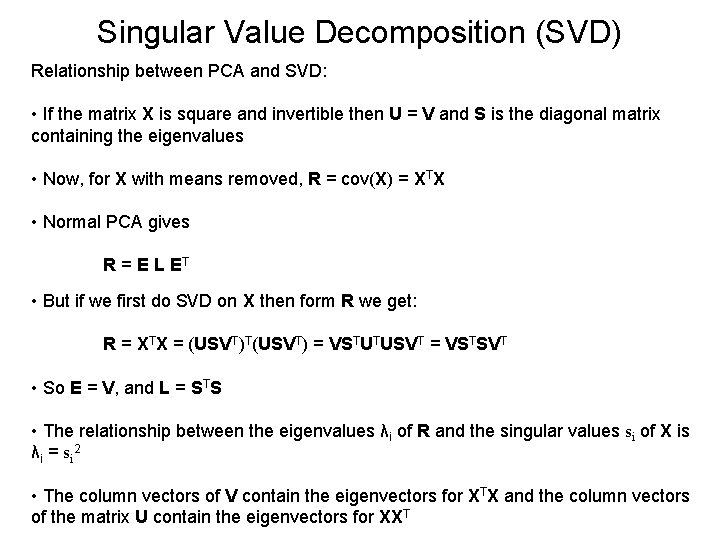
Singular Value Decomposition (SVD) Relationship between PCA and SVD: • If the matrix X is square and invertible then U = V and S is the diagonal matrix containing the eigenvalues • Now, for X with means removed, R = cov(X) = XTX • Normal PCA gives R = E L ET • But if we first do SVD on X then form R we get: R = XTX = (USVT)T(USVT) = VSTUTUSVT = VSTSVT • So E = V, and L = STS • The relationship between the eigenvalues λi of R and the singular values si of X is λi = si 2 • The column vectors of V contain the eigenvectors for XTX and the column vectors of the matrix U contain the eigenvectors for XXT

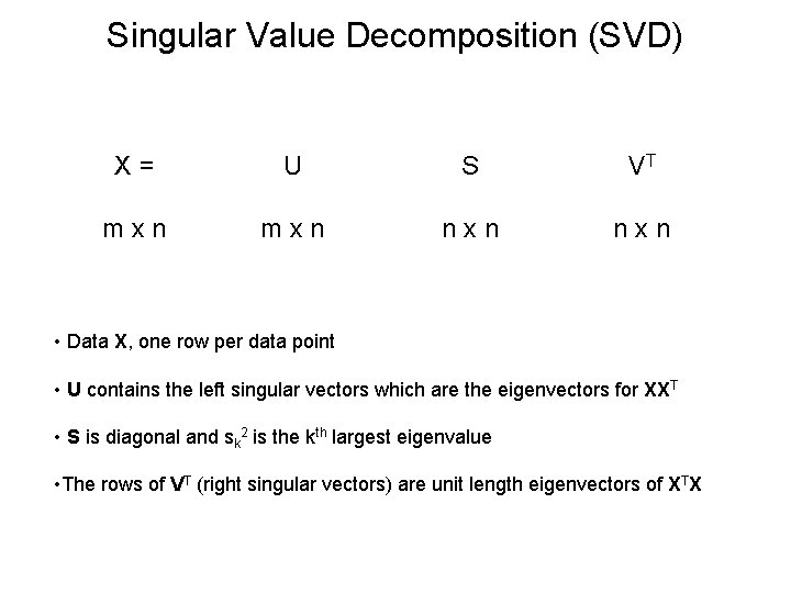
Singular Value Decomposition (SVD) X = U S VT m x n n x n • Data X, one row per data point • U contains the left singular vectors which are the eigenvectors for XXT • S is diagonal and sk 2 is the kth largest eigenvalue • The rows of VT (right singular vectors) are unit length eigenvectors of XTX

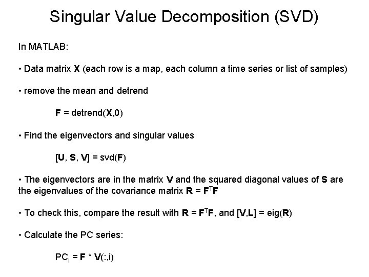
Singular Value Decomposition (SVD) In MATLAB: • Data matrix X (each row is a map, each column a time series or list of samples) • remove the mean and detrend F = detrend(X, 0) • Find the eigenvectors and singular values [U, S, V] = svd(F) • The eigenvectors are in the matrix V and the squared diagonal values of S are the eigenvalues of the covariance matrix R = FTF • To check this, compare the result with R = FTF, and [V, L] = eig(R) • Calculate the PC series: PCi = F * V(: , i)

Applications of PCA

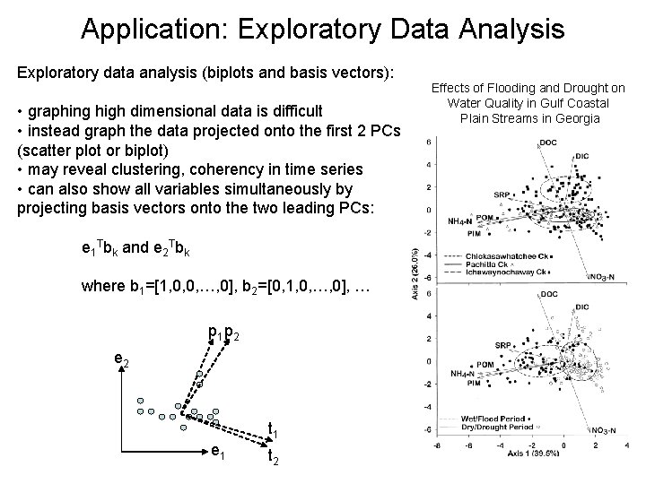
Application: Exploratory Data Analysis Exploratory data analysis (biplots and basis vectors): • graphing high dimensional data is difficult • instead graph the data projected onto the first 2 PCs (scatter plot or biplot) • may reveal clustering, coherency in time series • can also show all variables simultaneously by projecting basis vectors onto the two leading PCs: e 1 Tbk and e 2 Tbk where b 1=[1, 0, 0, …, 0], b 2=[0, 1, 0, …, 0], … p 1 p 2 e 2 t 1 e 1 t 2 Effects of Flooding and Drought on Water Quality in Gulf Coastal Plain Streams in Georgia

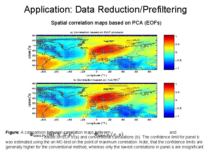
Application: Data Reduction/Prefiltering Spatial correlation maps based on PCA (EOFs) Figure: A comparison between correlation maps between and , based on EOFs (a) and conventional calculations (b). The confidence limit for panel b was estimated using the an MC-test on the point of maximum correlation. Note, that the confidence limits are generally higher for the conventional method, whereas only the lowest correlations in panel a are insignificant

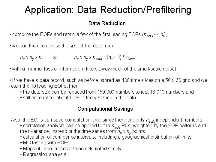
Application: Data Reduction/Prefiltering Data Reduction • compute the EOFs and retain a few of the first leading EOFs (neofs << nt), • we can then compress the size of the data from nx x ny x nt to nx x ny x neofs + (nt + 1) * neofs • with a minimal loss of information (filters away much of the small-scale noise). • If we have a data record, such as before, stored as 100 time slices on a 50 x 30 grid and we retain the 10 leading EOFs, then • the data size can be reduced from 150, 000 numbers to just 16, 010 numbers and • still account for about 90% of the variance in the data Computational Savings Also, the EOFs can save computation time since there are only neofs independent numbers. • correlation analysis can be applied to the neofs PCs, weighted by the EOF patterns and their variance, instead of the time series from nx x ny points. • calculation of confidence intervals, including a geographical distribution of limits • MC testing with EOFs • Maps of linear trends can be calculated simply • Regression analysis

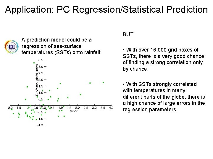
Application: PC Regression/Statistical Prediction A prediction model could be a regression of sea-surface temperatures (SSTs) onto rainfall: BUT • With over 16, 000 grid boxes of SSTs, there is a very good chance of finding a strong correlation only by chance. • With SSTs strongly correlated with temperatures in many different parts of the globe, there is a high chance of large errors in the regression parameters.

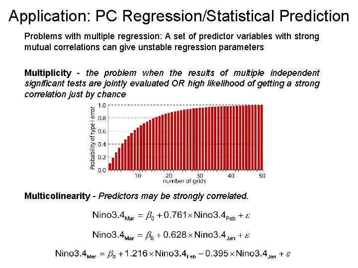
Application: PC Regression/Statistical Prediction Problems with multiple regression: A set of predictor variables with strong mutual correlations can give unstable regression parameters Multiplicity - the problem when the results of multiple independent significant tests are jointly evaluated OR high likelihood of getting a strong correlation just by chance Multicolinearity - Predictors may be strongly correlated.

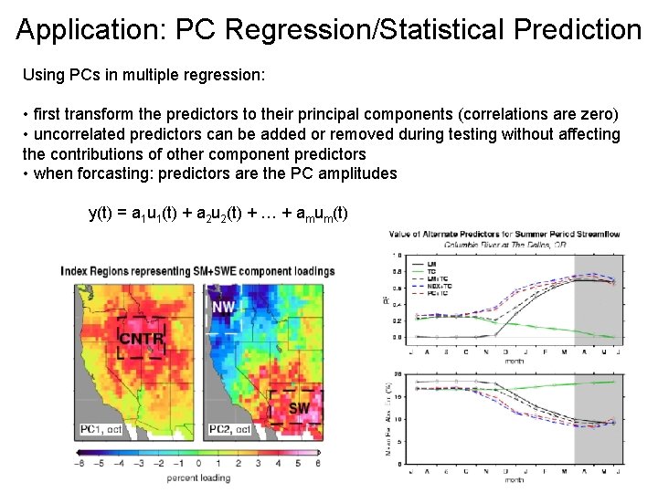
Application: PC Regression/Statistical Prediction Using PCs in multiple regression: • first transform the predictors to their principal components (correlations are zero) • uncorrelated predictors can be added or removed during testing without affecting the contributions of other component predictors • when forcasting: predictors are the PC amplitudes y(t) = a 1 u 1(t) + a 2 u 2(t) + … + amum(t)