PCA Lecture 3 Extensions of PCA and Related

PCA: Lecture 3 Extensions of PCA and Related Tools • Extended EOF (EEOF), Singular spectrum analysis (SSA), M-SSA • Canonical Correlation Analysis (CCA) • Others • Complex EOFs • Maximum Covariance Analysis • Principal Oscillation Patterns (POP) • Independent Component Analysis (ISA)

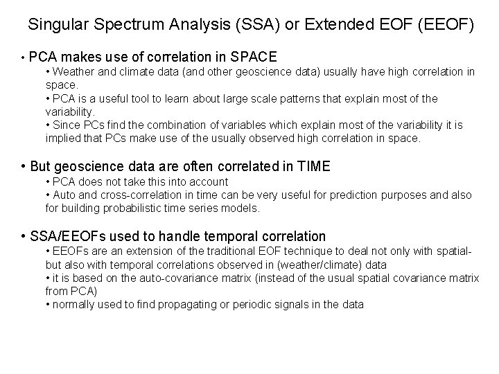
Singular Spectrum Analysis (SSA) or Extended EOF (EEOF) • PCA makes use of correlation in SPACE • Weather and climate data (and other geoscience data) usually have high correlation in space. • PCA is a useful tool to learn about large scale patterns that explain most of the variability. • Since PCs find the combination of variables which explain most of the variability it is implied that PCs make use of the usually observed high correlation in space. • But geoscience data are often correlated in TIME • PCA does not take this into account • Auto and cross-correlation in time can be very useful for prediction purposes and also for building probabilistic time series models. • SSA/EEOFs used to handle temporal correlation • EEOFs are an extension of the traditional EOF technique to deal not only with spatialbut also with temporal correlations observed in (weather/climate) data • it is based on the auto-covariance matrix (instead of the usual spatial covariance matrix from PCA) • normally used to find propagating or periodic signals in the data

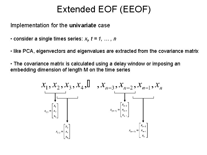
Extended EOF (EEOF) Implementation for the univariate case • consider a single times series: xt, t = 1, … , n • like PCA, eigenvectors and eigenvalues are extracted from the covariance matrix • The covariance matrix is calculated using a delay window or imposing an embedding dimension of length M on the time series

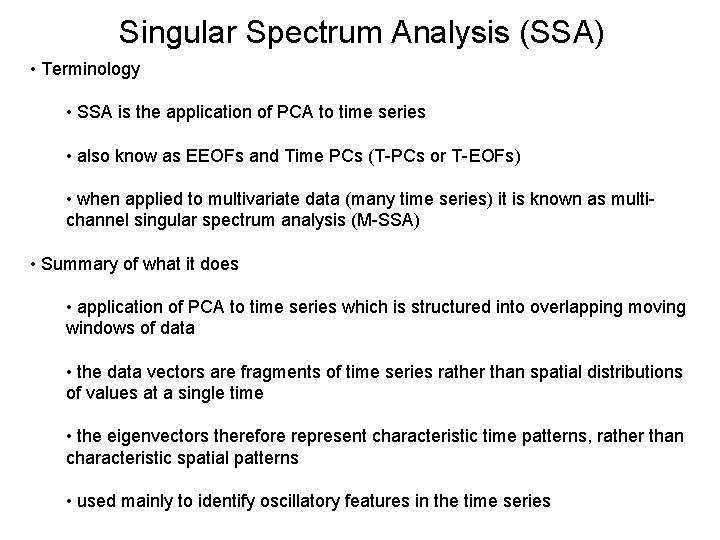
Singular Spectrum Analysis (SSA) • Terminology • SSA is the application of PCA to time series • also know as EEOFs and Time PCs (T-PCs or T-EOFs) • when applied to multivariate data (many time series) it is known as multichannel singular spectrum analysis (M-SSA) • Summary of what it does • application of PCA to time series which is structured into overlapping moving windows of data • the data vectors are fragments of time series rather than spatial distributions of values at a single time • the eigenvectors therefore represent characteristic time patterns, rather than characteristic spatial patterns • used mainly to identify oscillatory features in the time series

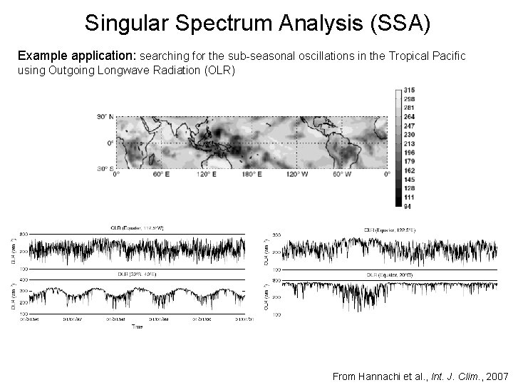
Singular Spectrum Analysis (SSA) Example application: searching for the sub-seasonal oscillations in the Tropical Pacific using Outgoing Longwave Radiation (OLR) From Hannachi et al. , Int. J. Clim. , 2007

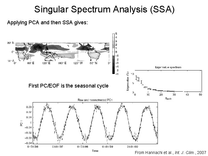
Singular Spectrum Analysis (SSA) Applying PCA and then SSA gives: First PC/EOF is the seasonal cycle From Hannachi et al. , Int. J. Clim. , 2007

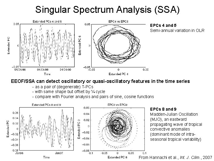
Singular Spectrum Analysis (SSA) EPCs 4 and 5 Semi-annual variation in OLR EEOF/SSA can detect oscillatory or quasi-oscillatory features in the time series - as a pair of (degenerate) T-PCs - with same shape but offset by ¼ cycle - compare with Fourier analysis and pairs of sine, cosine functions EPCs 8 and 9 Madden-Julian Oscillation (MJO), an eastward propagating wave of tropical convective anomalies (dominant mode of intraseasonal tropical variability) From Hannachi et al. , Int. J. Clim. , 2007

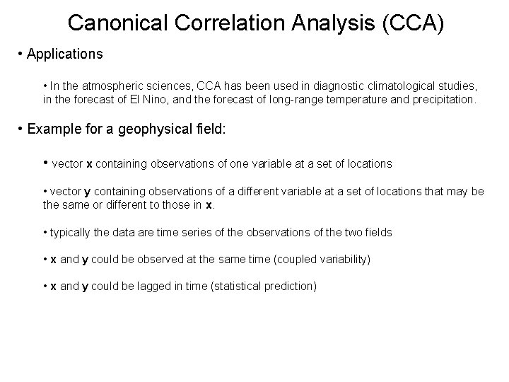
Canonical Correlation Analysis (CCA) • Definition of CCA • identifies a sequence of pairs of patterns in 2 multivariate data sets, and constructs sets of transformed variables by projecting the original data onto these patterns • Difference between PCA and CCA • PCA looks for patterns with a single multivariate dataset that represent maximum amounts of the variation in the data • In CCA, the patterns are chosen such that the projected data onto these patterns exhibit maximum correlation – while being uncorrelated with the projections onto any other pattern • In other words: CCA identifies new variables that maximize the inter-relationships between two data sets, in contrast to the patterns describing the internal variability within a single dataset from PCA. • Link to Multiple Regression • Can be thought of as an extension to multiple regression • instead of predicting a scalar y, we are predicting a vector y

Canonical Correlation Analysis (CCA) • Applications • In the atmospheric sciences, CCA has been used in diagnostic climatological studies, in the forecast of El Nino, and the forecast of long-range temperature and precipitation. • Example for a geophysical field: • vector x containing observations of one variable at a set of locations • vector y containing observations of a different variable at a set of locations that may be the same or different to those in x. • typically the data are time series of the observations of the two fields • x and y could be observed at the same time (coupled variability) • x and y could be lagged in time (statistical prediction)

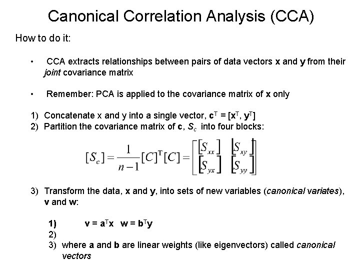
Canonical Correlation Analysis (CCA) How to do it: • CCA extracts relationships between pairs of data vectors x and y from their joint covariance matrix • Remember: PCA is applied to the covariance matrix of x only 1) Concatenate x and y into a single vector, c. T = [x. T, y. T] 2) Partition the covariance matrix of c, Sc into four blocks: 3) Transform the data, x and y, into sets of new variables (canonical variates), v and w: 1) v = a. Tx w = b Ty 2) 3) where a and b are linear weights (like eigenvectors) called canonical vectors

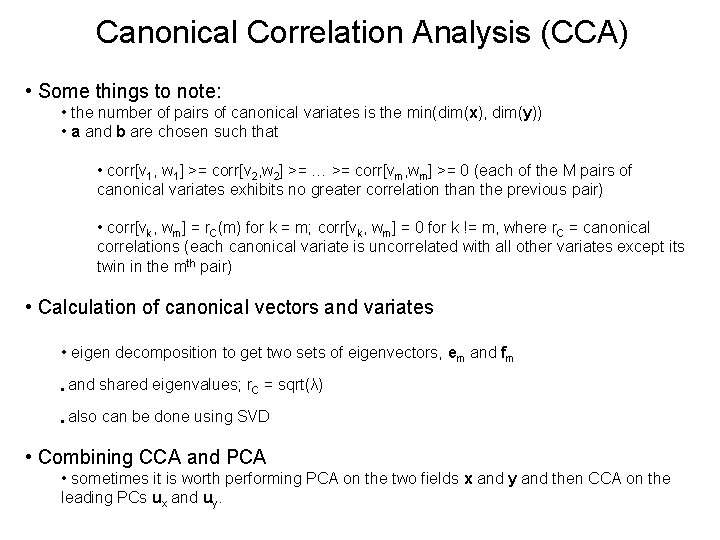
Canonical Correlation Analysis (CCA) • Some things to note: • the number of pairs of canonical variates is the min(dim(x), dim(y)) • a and b are chosen such that • corr[v 1, w 1] >= corr[v 2, w 2] >= … >= corr[vm, wm] >= 0 (each of the M pairs of canonical variates exhibits no greater correlation than the previous pair) • corr[vk, wm] = r. C(m) for k = m; corr[vk, wm] = 0 for k != m, where r. C = canonical correlations (each canonical variate is uncorrelated with all other variates except its twin in the mth pair) • Calculation of canonical vectors and variates • eigen decomposition to get two sets of eigenvectors, em and fm • and shared eigenvalues; r. C = sqrt(λ) • also can be done using SVD • Combining CCA and PCA • sometimes it is worth performing PCA on the two fields x and y and then CCA on the leading PCs ux and uy.

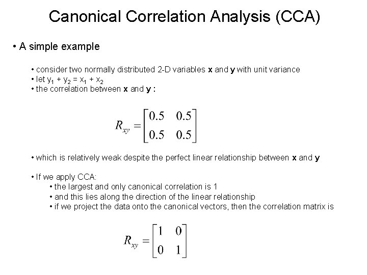
Canonical Correlation Analysis (CCA) • A simple example • consider two normally distributed 2 -D variables x and y with unit variance • let y 1 + y 2 = x 1 + x 2 • the correlation between x and y : • which is relatively weak despite the perfect linear relationship between x and y • If we apply CCA: • the largest and only canonical correlation is 1 • and this lies along the direction of the linear relationship • if we project the data onto the canonical vectors, then the correlation matrix is

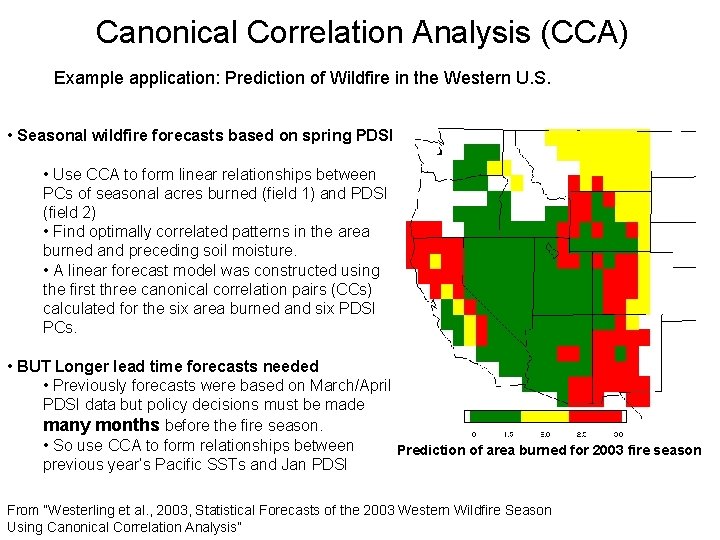
Canonical Correlation Analysis (CCA) Example application: Prediction of Wildfire in the Western U. S. • Seasonal wildfire forecasts based on spring PDSI • Use CCA to form linear relationships between PCs of seasonal acres burned (field 1) and PDSI (field 2) • Find optimally correlated patterns in the area burned and preceding soil moisture. • A linear forecast model was constructed using the first three canonical correlation pairs (CCs) calculated for the six area burned and six PDSI PCs. • BUT Longer lead time forecasts needed • Previously forecasts were based on March/April PDSI data but policy decisions must be made many months before the fire season. • So use CCA to form relationships between Prediction of area burned for 2003 fire season previous year’s Pacific SSTs and Jan PDSI From “Westerling et al. , 2003, Statistical Forecasts of the 2003 Western Wildfire Season Using Canonical Correlation Analysis”

Other Extensions and Some Relatives • Complex-EOF To extend the EOF analysis to the study of spatial structures that can propagate in time, one can perform a complex principal component analysis in the frequency domain. • Maximum Covariance Analysis (MCA) Finds linear combinations of two sets of vector data, x and y, that maximizes their covariance (CCA maximizes their correlation). • Independent Component Analysis (ICA) ICA seeks directions that are most statistically independent. i. e. that minimize the mutual information between the data. • Principal Oscillation Patterns (POP) POPs are used to examine the oscillation properties and spatial structure of dynamical processes in the atmosphere