DIY fractional polynomials Patrick Royston MRC Clinical Trials

DIY fractional polynomials Patrick Royston MRC Clinical Trials Unit , London 10 September 2010

Overview • Introduction to fractional polynomials • Going off-piste: DIY fractional polynomials • Examples

3

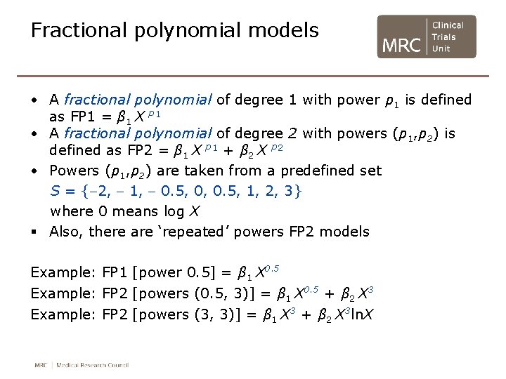
Fractional polynomial models • A fractional polynomial of degree 1 with power p 1 is defined as FP 1 = β 1 X p 1 • A fractional polynomial of degree 2 with powers (p 1, p 2) is defined as FP 2 = β 1 X p 1 + β 2 X p 2 • Powers (p 1, p 2) are taken from a predefined set S = { 2, 1, 0. 5, 0, 0. 5, 1, 2, 3} where 0 means log X § Also, there are ‘repeated’ powers FP 2 models Example: FP 1 [power 0. 5] = β 1 X 0. 5 Example: FP 2 [powers (0. 5, 3)] = β 1 X 0. 5 + β 2 X 3 Example: FP 2 [powers (3, 3)] = β 1 X 3 + β 2 X 3 ln. X

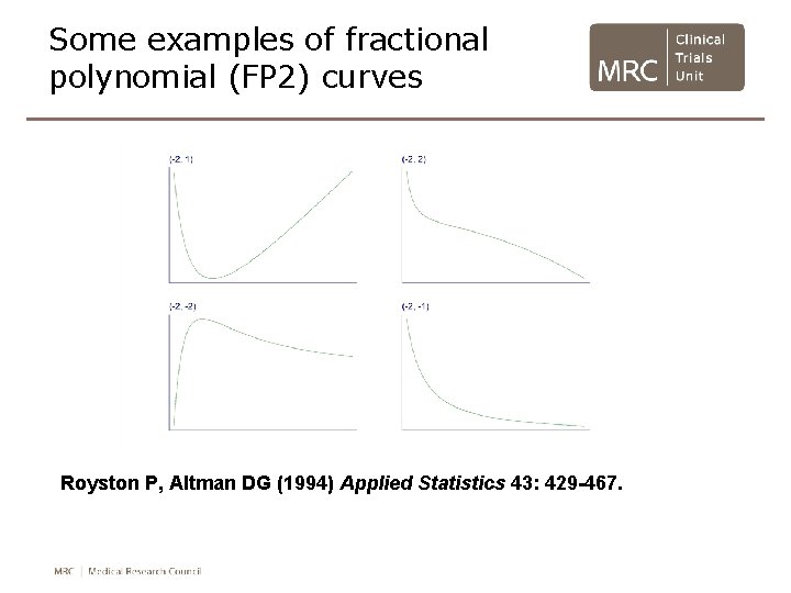
Some examples of fractional polynomial (FP 2) curves Royston P, Altman DG (1994) Applied Statistics 43: 429 -467.

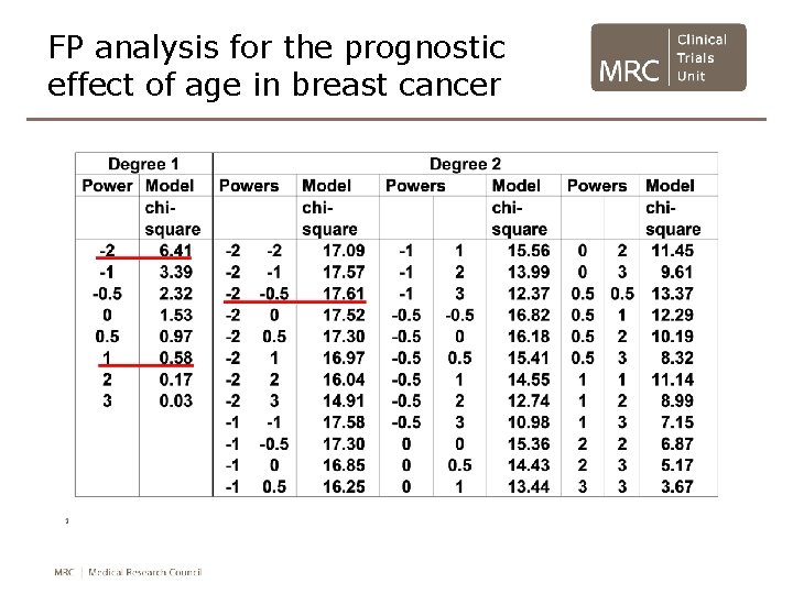
FP analysis for the prognostic effect of age in breast cancer

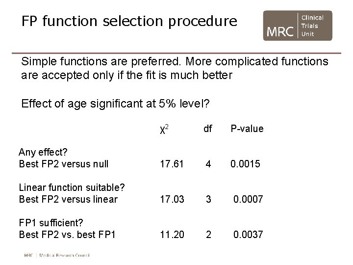
FP function selection procedure Simple functions are preferred. More complicated functions are accepted only if the fit is much better Effect of age significant at 5% level? χ2 df P-value Any effect? Best FP 2 versus null 17. 61 4 0. 0015 Linear function suitable? Best FP 2 versus linear 17. 03 3 0. 0007 FP 1 sufficient? Best FP 2 vs. best FP 1 11. 20 2 0. 0037

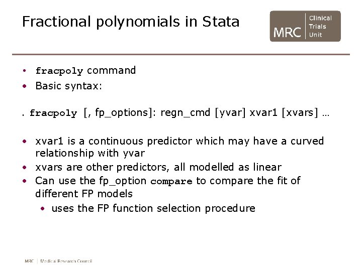
Fractional polynomials in Stata • fracpoly command • Basic syntax: . fracpoly [, fp_options]: regn_cmd [yvar] xvar 1 [xvars] … • xvar 1 is a continuous predictor which may have a curved relationship with yvar • xvars are other predictors, all modelled as linear • Can use the fp_option compare to compare the fit of different FP models • uses the FP function selection procedure

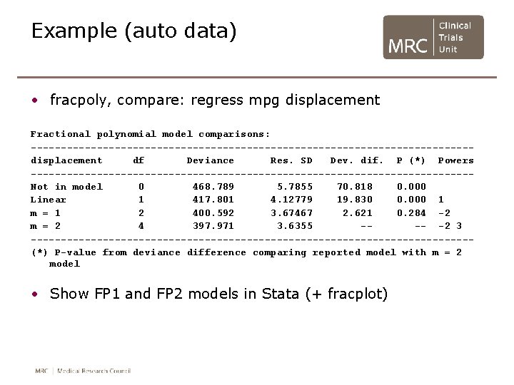
Example (auto data) • fracpoly, compare: regress mpg displacement Fractional polynomial model comparisons: -------------------------------------displacement df Deviance Res. SD Dev. dif. P (*) Powers -------------------------------------Not in model 0 468. 789 5. 7855 70. 818 0. 000 Linear 1 417. 801 4. 12779 19. 830 0. 000 1 m = 1 2 400. 592 3. 67467 2. 621 0. 284 -2 m = 2 4 397. 971 3. 6355 --- -2 3 -------------------------------------(*) P-value from deviance difference comparing reported model with m = 2 model • Show FP 1 and FP 2 models in Stata (+ fracplot)

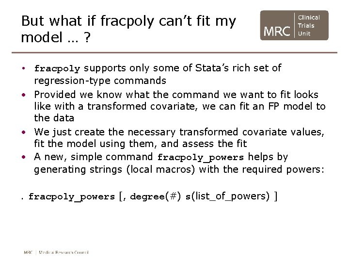
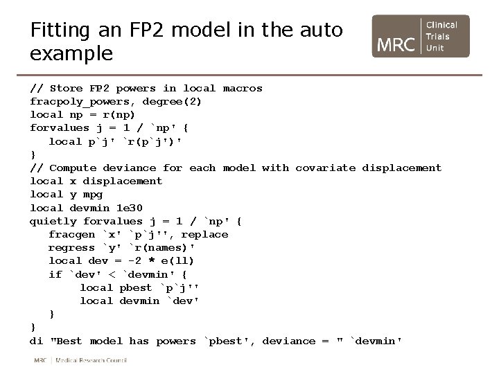
But what if fracpoly can’t fit my model … ? • fracpoly supports only some of Stata’s rich set of regression-type commands • Provided we know what the command we want to fit looks like with a transformed covariate, we can fit an FP model to the data • We just create the necessary transformed covariate values, fit the model using them, and assess the fit • A new, simple command fracpoly_powers helps by generating strings (local macros) with the required powers: . fracpoly_powers [, degree(#) s(list_of_powers) ]

Fitting an FP 2 model in the auto example // Store FP 2 powers in local macros fracpoly_powers, degree(2) local np = r(np) forvalues j = 1 / `np' { local p`j' `r(p`j')' } // Compute deviance for each model with covariate displacement local x displacement local y mpg local devmin 1 e 30 quietly forvalues j = 1 / `np' { fracgen `x' `p`j'', replace regress `y' `r(names)' local dev = -2 * e(ll) if `dev' < `devmin' { local pbest `p`j'' local devmin `dev' } } di "Best model has powers `pbest', deviance = " `devmin'

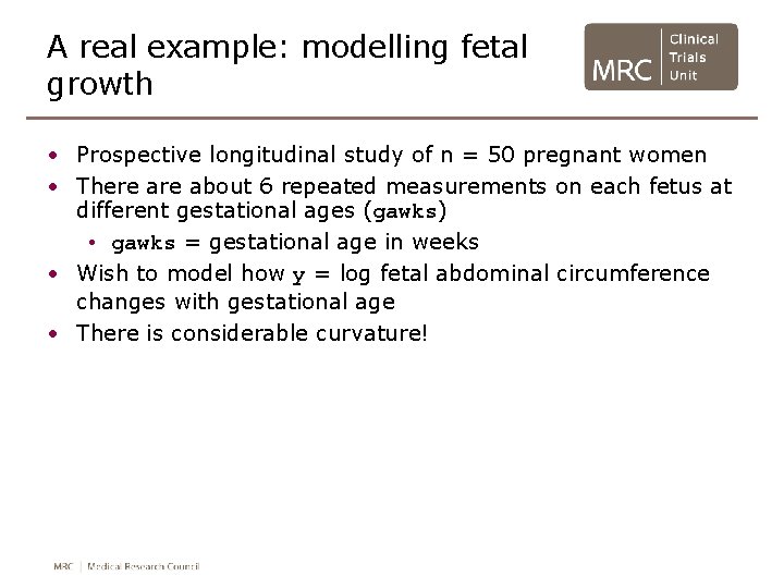
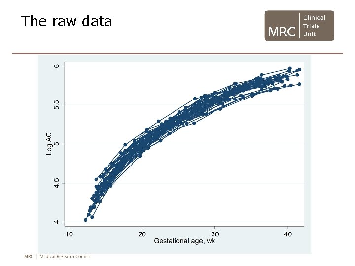
A real example: modelling fetal growth • Prospective longitudinal study of n = 50 pregnant women • There about 6 repeated measurements on each fetus at different gestational ages (gawks) • gawks = gestational age in weeks • Wish to model how y = log fetal abdominal circumference changes with gestational age • There is considerable curvature!

The raw data

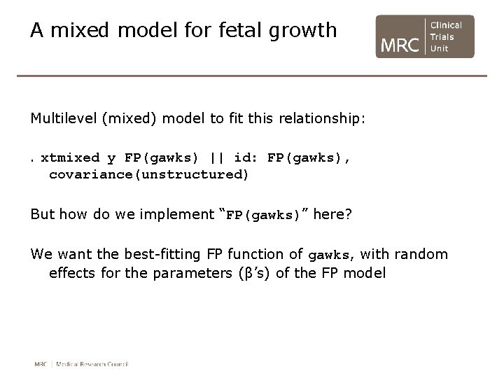
A mixed model for fetal growth Multilevel (mixed) model to fit this relationship: . xtmixed y FP(gawks) || id: FP(gawks), covariance(unstructured) But how do we implement “FP(gawks)” here? We want the best-fitting FP function of gawks, with random effects for the parameters (β’s) of the FP model

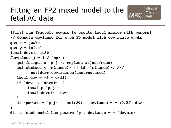
Fitting an FP 2 mixed model to the fetal AC data [First run fracpoly_powers to create local macros with powers] // Compute deviance for each FP model with covariate gawks gen x = gawks gen y = ln(ac) local devmin 1 e 30 forvalues j = 1 / `np' { qui fracgen x `p`j'', replace adjust(mean) qui xtmixed y `r(names)' || id: `r(names)', /// nostderr covariance(unstructured) local dev = -2 * e(ll) if `dev' < `devmin' { local p `p`j'' local devmin `dev' } di "powers = `p`j''" _col(20) " deviance = " %9. 3 f `dev' } di _n "Best model has powers `p', deviance = " `devmin'

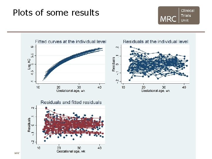
Plots of some results

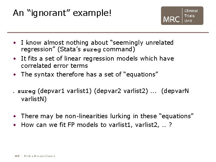
An “ignorant” example! • I know almost nothing about “seemingly unrelated regression” (Stata’s sureg command) • It fits a set of linear regression models which have correlated error terms • The syntax therefore has a set of “equations”. sureg (depvar 1 varlist 1) (depvar 2 varlist 2). . . (depvar. N varlist. N) • There may be non-linearities lurking in these “equations” • How can we fit FP models to varlist 1, varlist 2, … ?

Example: modelling learning scores Stata FAQ from UCLA (http: //www. ats. ucla. edu/stata/faq/sureg. htm): What is seemingly unrelated regression and how can I perform it in Stata? Example: High School and Beyond study

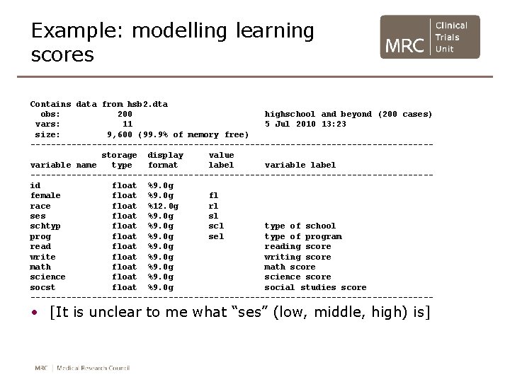
Example: modelling learning scores Contains data from hsb 2. dta obs: 200 highschool and beyond (200 cases) vars: 11 5 Jul 2010 13: 23 size: 9, 600 (99. 9% of memory free) ---------------------------------------storage display value variable name type format label variable label ---------------------------------------id float %9. 0 g female float %9. 0 g fl race float %12. 0 g rl ses float %9. 0 g sl schtyp float %9. 0 g scl type of school prog float %9. 0 g sel type of program read float %9. 0 g reading score write float %9. 0 g writing score math float %9. 0 g math score science float %9. 0 g science score socst float %9. 0 g social studies score ---------------------------------------- • [It is unclear to me what “ses” (low, middle, high) is]

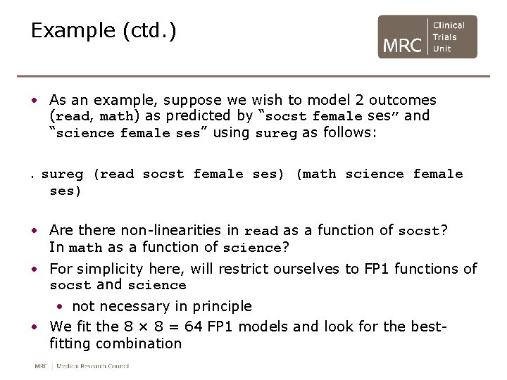
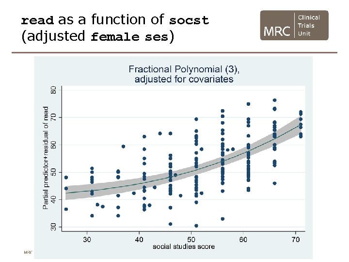
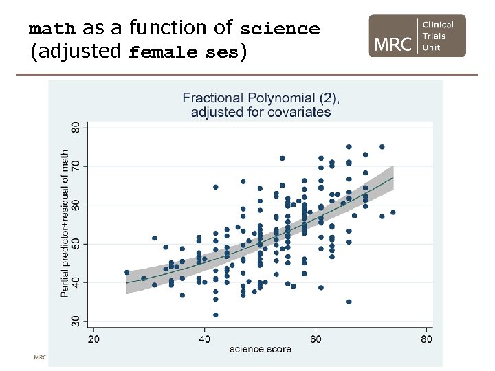
Example (ctd. ) • As an example, suppose we wish to model 2 outcomes (read, math) as predicted by “socst female ses” and “science female ses” using sureg as follows: . sureg (read socst female ses) (math science female ses) • Are there non-linearities in read as a function of socst? In math as a function of science? • For simplicity here, will restrict ourselves to FP 1 functions of socst and science • not necessary in principle • We fit the 8 × 8 = 64 FP 1 models and look for the bestfitting combination

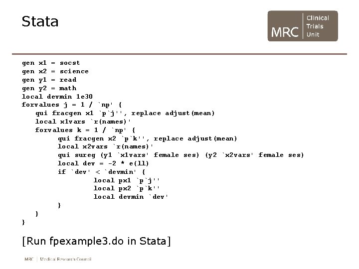
Stata gen x 1 = socst gen x 2 = science gen y 1 = read gen y 2 = math local devmin 1 e 30 forvalues j = 1 / `np' { qui fracgen x 1 `p`j'', replace adjust(mean) local x 1 vars `r(names)' forvalues k = 1 / `np' { qui fracgen x 2 `p`k'', replace adjust(mean) local x 2 vars `r(names)' qui sureg (y 1 `x 1 vars' female ses) (y 2 `x 2 vars' female ses) local dev = -2 * e(ll) if `dev' < `devmin' { local px 1 `p`j'' local px 2 `p`k'' local devmin `dev' } } } [Run fpexample 3. do in Stata]

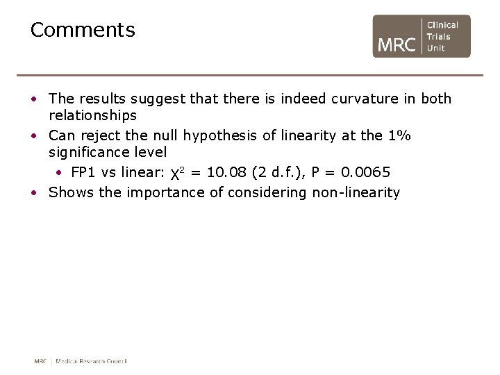
Comments • The results suggest that there is indeed curvature in both relationships • Can reject the null hypothesis of linearity at the 1% significance level • FP 1 vs linear: χ2 = 10. 08 (2 d. f. ), P = 0. 0065 • Shows the importance of considering non-linearity

read as a function of socst (adjusted female ses)

math as a function of science (adjusted female ses)

Conclusions • Fractional polynomial models are a simple yet very useful extension of linear functions and ordinary polynomials • If you are willing to do some straightforward do-file programming, you can apply them in a bespoke manner to a wide range of Stata regression-type commands and get useful results • For (much) more, see Royston & Sauerbrei (2008) book