Course Overview cmpt 307 Two ancient problems Factoring

Course Overview cmpt 307

Two ancient problems • Factoring: Given a number N , express it as a product of its prime factors. • Primality: Given a number N, determine whether it is a prime. • Factoring is hard. Despite centuries of efforts the fastest methods for factoring a number N take time exponential in number of bits of N. • On the other hand, we can efficiently test whether N is prime!

Elementary Number Theory • Prime Numbers – building block of integers – every positive integer can be written uniquely as a product of prime numbers – difficult to write large integers as a product of primes.

Primality Testing and Factorization

Basic arithmetic • Addition – The sum of any three single-digit numbers is at most two digit long. – The cost of each addition of two integers m and n is O(log m +log n).

Basic arithmetic • Multiplication and Division – multiplying two integers m and n cost O(log m. log n). – Can do better with divide-and-conquer.

Modular arithmetic • Repeated addition and multiplication can get the result cumbersomely large. • Modular arithmetic is a system for dealing with restricted range of numbers.

Exponentiation • In cryptosystem, it is necessary to compute xy mod N for values of x, y, and N that are several hundred bits long. • Like to evaluate 2 (19*(524288)) mod (N).

Exponentiation xy mod n = (x mod n)(y mod n) mod n xy mod n = (x mod n)y mod n

Modular exponentiation number of bits to represent xy = O(ylog x) number of bits to represent xy mod N is O(log N).

Euclid’s algorithm (discovered 2000 years ago) • gcd(a, b) // assume that a > b – If b=0 then return a. – Compute r = a mod b – return gcd(b, r) • This takes logarithmic time. – after every two iterations, the largest number gets reduced by a half at least.

Important Property • Given any two integers a and b, there exist integers x and y, such that ax + by = gcd(a, b).

Least Common Multiple (lcm)

Modular division • In real arithmetic, every number a (≠ 0) has an inverse, 1/a. • Multiplying by 1/a is the same as dividing by a. • In modular arithmetic we can make a similar definition: x is a multiplicative inverse of “a modulo b” iff ax = 1 (mod b). • Theorem: The inverse of a modulo b exists and is unique iff a is relatively prime to b, i. e. gcd(a, b) = 1. – gcd(a, b) = 1 implies ax + by = 1 for some integer x and y – ax = 1 – by implies ax ≡ 1 (mod b).

Solve the equation 247 x + 91 y = 39 • • We need to find an x and y (integers) We find that gcd(247, 91) = 13. Since 13 divides 39, we have a solution. We can write 3 × 247 – 8 × 91 = 13 or 3 × 19 − 8 × 7 = 1 or 3 × 19 – 19 × 7 × t + 19 × 7 × t – 8 × 7 = 1 or 19 ( 3 – 7 t) + 7 ( 19 t -8) = 1 for any integer t • Therefore, x = 3 -7 t and y = 19 t – 8. (ans)

Analysis of algorithms Chapter 2

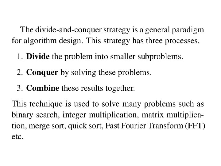
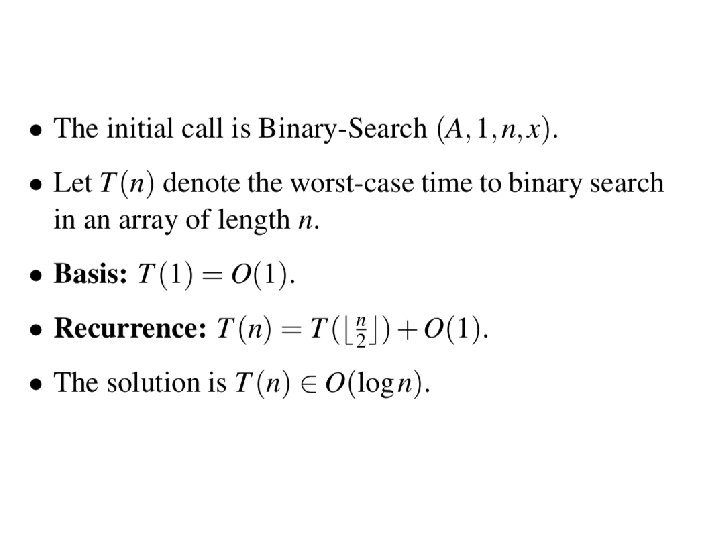
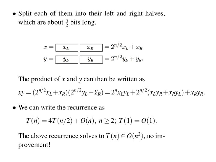
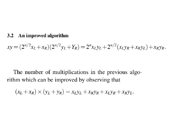
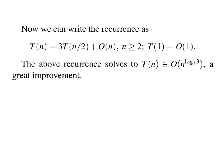
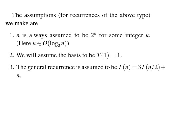
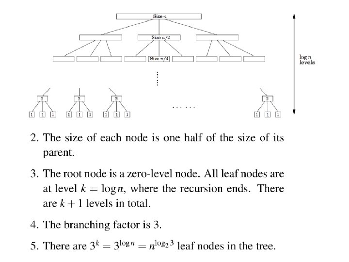
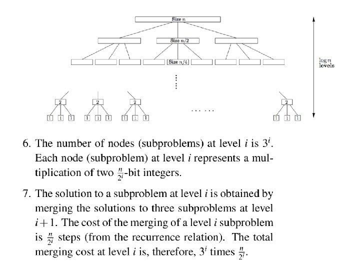
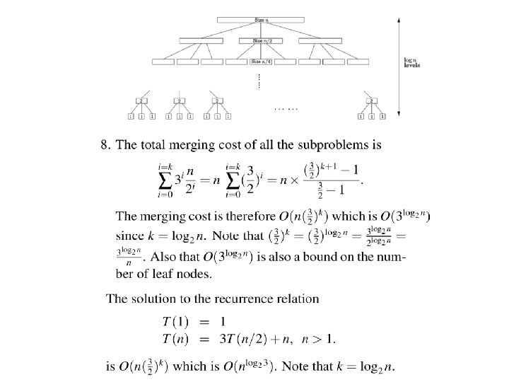
Divide-and-conquer Chapter 2

Part A

Part B

Graphs (Chapter 3)

Some examples • Connected graph • Complete graph

Some examples • Disconnected graph

Some examples • Edge-weighted graph

Graph Terminology • When analyzing algorithms on a graph, there are usually two parameters we care about: – The number of nodes n. (n = |V|) – The number of edges m, (m = |E|) • Note that m = O(n 2). • A graph is dense if m = Θ(n 2). A graph is called sparse if it is not dense.

Storage space: O(n 2)

Storage space: O(n+m)

Adjacency matrix benefit • The biggest convenience is that the presence of a particular edge can be checked in constant time. • Any algorithm that uses adjacency matrix structure to store a graph has Ω(n 2) lower bound. This is true even if |E| is O(n).

Adjacency lists benefits • The storage space requirement is O(n + m), which is optimal in the sense that no other representation taking less than this amount is possible. • Checking of for an edge is no longer a constant time operation. • Iterating through all the neighbors of a vertex is now easy. • An algorithm on a graph runs in linear time if the running time of the algorithm is O(n + m).

Relative advantages of adjacency lists and matrices (From the book: The Algorithm Design Manual by Skienna)

Depth-first search (DFS) in undirected graph • DFS is a versatile linear time procedure to traverse (explore) a graph. • The undirected graph G=(V, E) is represented by an adjacency list. • DFS traverses a graph G = (V, E) in a systematic manner revealing a wealth of information about a graph.

An example parent[A] = nil parent[B] = A parent[E] = A parent[I] = E parent[j] = I • The solid edges are actually those that are traversed, each of which is effected by a call to explore and led to the discovery of a new vertex. These edges form a tree. The edges are call DFS tree edges. • Tree edges are { (parent[u], u)| u, parent[u] is not nill}

dfs(G) • The explore procedure visits only the portion of the graph reachable from its starting point. • To examine the rest of the graph, we need to restart the procedure elsewhere, at some vertex that has not yet been visited.

Procedure dfs(G)

An example

Analysis of dfs(G) • The worst case running time is O(|V|+|E|). • DFS algorithm is optimal.

Interesting observation of time intervals • The time intervals have interesting and useful properties with respect to a depth-first search. • Who is an ancestor in the DFS tree? • How many descendants? • How many connected components in G?

• • Vertices are picked in lexicographic order. A is the root of the search tree; everything else is its descendants. E has descendants F, H, G, and conversely, is an ancestor of these three nodes. C is the parent of D

Types of edges • Tree edges: Edges lead from a node to visit its children. The resulting tree could be disconnected (forest). • Forward edges: Edges lead from a node to a nonchild descendant in DFS tree. • Back edges: Edges lead to an ancestor in the DFS tree • Cross edges: Edges lead to neither descendant nor ancestor.

Summary of the various possibilities for an edge (u, v)

Directed acyclic graphs (DAGs) • A graph without a cycle is called acyclic. • G is a DAG if and only if its depth-first search reveals no back edge. This can therefore be tested in optimal O(|V| + |E|) time. In a DAG, every edge leads to a vertex with lower exit (post) number. • DAGs are good for modeling hierarchies and temporal dependencies: course prerequisites, task dependencies etc.

Strongly Connected Components • Let G = (V, E) be a directed graph. • A strongly connected component (or SCC) of G is a subset C of V with the following properties: – C is not empty. – For any u, v C: u and v are strongly connected. – For any u C, v V – C: u and v are not strongly connected.

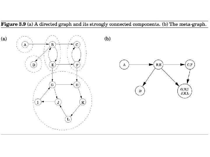
A directed graph and its strongly connected components

An important property • The condensation (meta) graph GSCC of any directed graph G is a dag. • Every dag has at least one source node and at least one sink node.

Identify a source strongly connected component • Perform DFS(G) • Find the node with the largest exit (post) time stamp.

Identify a source strongly connected component z lies in a strongly connected component which is a source node in the condensation graph GSCC. • Perform DFS(G) • Find the node z with the largest exit (post) time stamp.

Determine the SCC that contains z z z GSCC • • (GSCC) R Perform DFS on GR from node z where GR is obtained from G = (V, E) by reversing the direction of each edge of G. The search ends after finding the component containing z. The time spent to find this component is proportional to the size of the component. Remove all the nodes from G, reachable from z. Let G’ be the reduced graph.

Repeat the process after removing a component (G’)SCC • • • ((G’)SCC)R Select the next vertex z of G’ with the largest exit time stamp. z now lies in the component which is a source node of (G’)SCC. In the figure it is either B or E. We find all the vertices reachable from z’. These vertices form a strongly connected component.

Algorithm to computing strongly connected components • G is the given directed graph. – – Run DFS on G. Record the exit (post) time stamp of each node. Compute GR Run DFS on GR always starting from the node with the largest exit time stamp. • Since GR can be computed in linear time, the above algorithm runs in linear O(|V| + |E|) time.

Finding Cycles • In an undirected graph, the absence of nontree edges imply nonexistence of cycles. (why? ) • This can be tested by the DFS of the graph.

Topological Sorting • Topological sorting is the most important operation on DAGs. • It orders the vertices on a line such that all directed edges go from left to right. • Such an ordering cannot exist if the graph contains a directed cycle. • The ordering gives us a sequence of processes which can be executed honoring the precedence relation.

Shortest Paths (Chapter 4)

An application: Six degrees of separation Source node The numbers on nodes indicate the distances of the nodes from the source node.

Source node

Source node Principle of optimality: If node A lies on the shortest path from the source node S to B then d (S, B) = d (S, A) + d ( A, B).

General Idea of BFS • Proceed outward from the source node s in ``layers’’. – The first layer is all nodes of distance 0. – The second layer is all nodes of distance 1. – The third layer is all nodes of distance 2. – etc. • This gives rise to breadth-first search.

We keep only edges (thick ones) that correspond to parent field of some vertex.

DFS vs. BFS • Input: • Idea: – A Graph G = (V, E) (directed or undirected) – No source vertex given! – Explore the edges of G to “discover” every vertex in V starting at the most current visited node – Search may be repeated from multiple sources • Output: – 2 timestamps on each vertex: pre[v], post[v] – DFS forest • O(|V|+|E|) BFS – A graph G = (V, E) (directed or undirected) – A source vertex s V – Explore the edges of G to “discover” every vertex reachable from s, taking the ones closest to s first • Output: – d[v] = distance (smallest # of edges, or shortest path) from s to v, for all v V – BFS tree • O(|V|+|E|) 93

Using Array Implementations • O(|V|(Tins + Tex) + |E| Tdec) • Implement priority queue with an unsorted array: – – Tins = O(1), Tex = O(|V|), Tdec = O(1) total time is O(|V|2) 94

Edges have (positive) lengths • Breadth-first search treats all edges as having the same length. • In reality the edges have lengths, and we are interested in computing shortest paths. • Our graph is a weighted graph G = (V, E) where each edge e = (u, v) of E has length le or we will sometime also write l(u, v) or luv.

An intuitive description of Dijkstra’s algorithm • We are given a weighted graph G = (V, E), and interested in computing the shortest paths from s (source node). • We drop a huge colony of ants on to the source node s time 0. • They move from there and follow all possible paths through the graph at a rate of one unit per second. • The first one to reach the node v will do so at time dist(s, v). • dist(s, v) is the shortest distance from s to v.

Three operations on the schedule 1. Remove the entry with earliest time (this happens once for each node). 2. Add a new entry (this happens once for each entry) 3. Decrease the time associated with an existing entry (this happens at most once for each edge)

Using Array Implementations • O(|V|(Tins + Tex) + |E| Tdec) • Implement priority queue with an unsorted array: – – Tins = O(1), Tex = O(|V|), Tdec = O(1) total time is O(|V|2) 98

Running Time using Binary Heaps • O(|V|(Tins + Tex) + E Tdec) • If priority queue is implemented with a binary heap, then – Tins = Tex = Tdec = O(log |V|) – total time is O(|E| log |V|) 99

Running Time using Fibonacci Heaps • O(|V|(Tins + Tex) + E Tdec) • If priority queue is implemented with a Fibonacci heap, then – Tex = O(log |V|) – Tins = Tdec = O(1) – total time is O(|V| log |V| + |E|) 100

Performance Summary • Choice of priority queue implementation directly affects performance. • 2, 000 vertices, 1 million edges: heap 2 -3 times slower than array • 100, 000 vertices, 1 million edges: heap gives 500 x speedup • 1 million vertices, 2 million edges: heap gives 10, 000 x speedup. • array implementation is better for dense graph • heap is better for sparse graph

Shortest paths in the presence of negative edges • This property is no longer holds when edge length is allowed to be negative. Source A 2 8 5 C B Destination D -7 • Dijkstra’s algorithm still returns the path <A, C, D> as the shortest path from source node to destination node. However, this is incorrect. • Negative edge weights present problems for Dijkstra’s algorithm.

Shortest paths in the presence of negative cycles • A bigger problem is negative cycles like the one below, since this means that there doesn’t exists a true shortest paths. Source A -10 3 15 C B Destination D 5 • We can make the shortest paths as small as possible.

Bellman-Ford Algorithm • Handles graphs with negative edge weights. • It will return the same output as Dijkstra’s for any graphs with positive weights, but run slower.

Edge update v u Update (relaxation) sets dist(v) to the length of a shorter path from s to v.

Bellman-Ford algorithm • Running time is O(|E||V|). • Invariant: At end of phase i, dist(v) ≤ length of any path from s to v using at most I edges. • Theorem: If there are no negative cycles, upon termination, dist(v) is the length of the shortest path from s to v. • Observation: If dist(v) doesn’t change during phase i, there is no need to relax any edge leaving v in phase i+1.

Negative cycles • It can be tested if a given graph has a negative cycle. • Check if Bellman-Ford algorithm updates dist(v) for any v in phase |V|. If it does, the graph has a negative cycle. (why? )

Shortest paths in dags • • There is no cycle. Edge weights could be negative. We still cannot use Dijkstra’s algorithm. We can use Bellman-Ford algorithm. – Running time is O(|E||V|) – For dense graphs this is O(|V|3). • We can reduce the complexity to O(|V| + |E|).

Shortest paths in dags • Use the topological order of the vertices of the dags. (Can be done in linear time) – dist(s) = 0 – Determine the topological order of the vertices. (Also known as Linearize G) – for each vertex u of V, in linearized order for all edges (u, v), radiating from u: update(u, v)

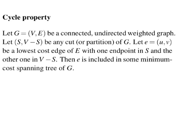
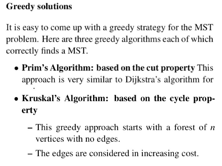
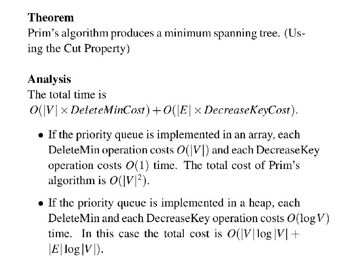
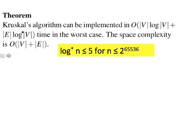
Greedy Algorithm Chapter 5

Dynamic Programming (DP) Chapter 6

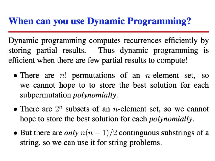
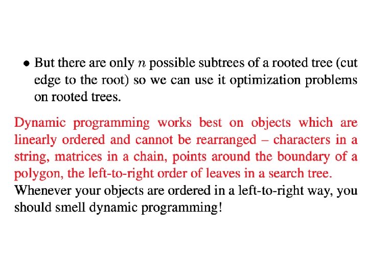
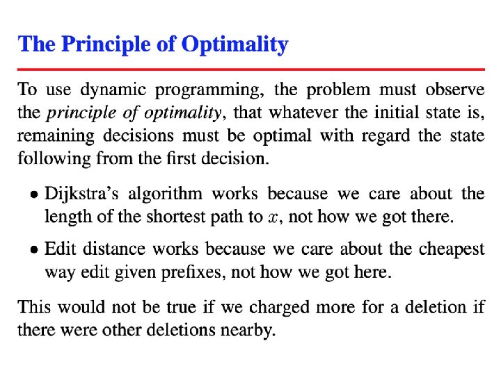
What is DP? • It is a ``method for solving complex problems by breaking them down into simpler subproblems’’.

Three steps for solving DP problems 1. Define subproblems 2. Formulate the recurrence that relates the subproblems 3. Recognize and solve the base cases. Each step is very important

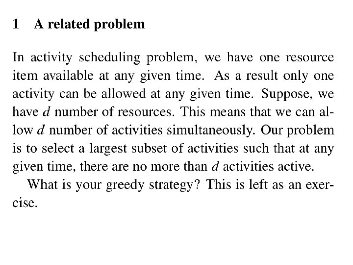
Weghted activity selection problem • Given a set S = {a 1, a 2, …, an} activities. • Activity ai has a start time si and a finish time fi. • Each activity ai has a value, or weight vi. • Two intervals are compatible if they do not overlap. • The problem is to select a subset of mutually compatible activities of largest total values.

Find the recurrence for Opt(i) • Define p(j), for an activity aj, to be the largest index i < j such that activities ai and aj are compatible.

Define subproblems: • Let Ai = {a 1, a 2, …, ai} be the set of first i activities. • Let Opt(i) be the total values of the optimal solution of the problem for the activities of Ai.

Find the recurrence for Opt(i) • Consider an optimal solution Opt(i) of Ai. – Opt(i) contains ai : Opt(i) = Opt(p(i)) + vi – Opt(i) does not contain ai : Opt(i) = Opt(i-1) • We get the recurrence by combining both the possibilities: – Opt(i) = max{ Opt(p(i)) + vi , Opt(i-1) } • Given Opt(i), how do we know whether ai is in Opt(i)? – ai is in Opt(i) if Opt(p(i)) + vj ≥ Opt(i-1).

Solve the base cases • The base case is Opt(0) = 0 • We can also say that Opt(1) = v 1.

Modified (memoized) Compute-Opt(j) (linear time) • Initialize an array Opt[]; – Opt[0] = 0; Opt[1. . n] undefined • Compute-Opt(j){ if Opt[j] is computed before, return Opt[j]; else Opt[j] = max(vj + Compute-Opt(p(j)), Compute-Opt(j-1)); return Opt[j]; } • The complexity of the algorithm is linear assuming that the intervals are already sorted by their finish times.

Iterated algorithm (bottom up) • Iterated-Compute-Opt(j) Opt[0] = 0; for (i = 1; I ≤ n; i++){ Opt[i] = max{ vi + Opt[p(j)], Opt[i-1]} } • Clearly, the algorithm is linear. • Memoized version is also linear. • Memoized version will take more time to compute due to the overhead cost of the recursion. • Memoized version is easier to code.

Finding the solution once Opt[. ] is known. • Find-Solution(j){ If j=0 Print nothing; else if vj + Opt[p(j)] ≥ Opt[j-1] { Print aj; Find-Solution(p(j)); } else Find-Solution(j-1); }

Shortest paths in DAGs • The graph G=(V, E) is directed, acyclic, weighted (possibly negative cost). • We can order the vertices (Using a DFS) on a line such that the directed edges can be drawn from the left to the right. (Topological ordering) • The leftmost vertex is a source and the rightmost vertex is a sink.

Shortest paths in DAGs • The shortest paths from the leftmost vertex to all the other nodes can be computed using Bellman-Ford algorithm. • The complexity is O(|V| + |E|) if the edges are ordered from left to right. Only two iterations are needed.

DP solution • Find the recurrence: – In the figure, the preceding vertex of the shortest path to D is either B or C. – Therefore, dist(D) = min{ dist(C) + 3, dist(B) +1} – A similar relation can be written for every node. • In general: dist[(v)] = min e=(u, v){dist(u) + ce} – ce is the cost of edge e pointing to v.

DP solution • Solve the base case: – dist(v 1) = 0;

DP solution • Find the recurrence: – In the figure, the preceding vertex of the shortest path to D is either B or C. – Therefore, dist(D) = min{ dist(C) + 3, dist(B) +1} – A similar relation can be written for every node. • In general: dist[(v)] = min e=(u, v){dist(u) + ce} – ce is the cost of edge e pointing to v.

Memoized-Solution (Top down) • The total cost of • memoized-dist(vj) computing the if vj = v 1 then shortest paths dist[vj] = 0 from the source return dist[vj] vertex to all the else other vertices in a if dist[vj] is computed before then DAG is O(|V|+|E|) return dist[vj]; else if vj has no incoming edge then dist[vj] = ∞ else dist[vj] = (dist[v] + ce) return dist[vj] • The total cost is O(in-degree of vj)

The Knapsack Problem • Input – Capacity W – n items with weights wi and values vi • Output: a set of items S such that • the sum of weights of items in S is at most W • and the sum of values of items in S is maximized

0 -1 Knapsack An item can either be picked or left. It cannot be picked partially. For example gold coins, diamond rings, TV etc.

DP solution • Define subproblems: – K(w, j) = maximum value achievable using a knapsack of capacity w and items 1 … j – Number of subproblems = n. W K(w, j), 0 ≤ w ≤ W, 0 ≤ j ≤ n – Number of subproblems is exponential in the input length of W.

DP solution • Find recurrence relation: – building larger subproblems by combining smaller subproblems – Want to solve K(w, j) – The optimal solution contains either item j or does not contain item j – If it contains item j, K(w, j) = vj + K(w – wj, j-1) – If it does not contain item j, K(w, j) = K(w, j-1) – Combining: K(w, j) = max {vj + K(w – wj, j-1), K(w, j-1)} • The cost of the optimal solution to the knapsack problem is K(W, n)

DP solution • Find base cases – K(0, j) = 0 for all j – K(w, 0) = 0 for all w.

Memoized-Solution (Top down) • memoized-K(w, j) if w = 0 then return 0; if j = 0 then return 0; else if wj > w then return K(w, j-1); if k[w, j] is computed before then return K[w, j]; else return max(K(w-wj, j-1) + vj, K(w, j-1)); • The total cost is # of subproblems which is O(n. W).

DP solution • The running time of the algorithm is O(n. W) • The running time is exponential in the input length of W, but not in the number of items. • The algorithm is a pseudo polynomial time algorithm.

Memoized-Solution (Top down) • memoized-output(w, j) if w ≤ 0 then return; if j = 0 then return; else if K(w, j) = K(w, j-1) then memoized-output(w, j-1); else Print j; memoized-output(w-wj, j-1); • The total cost is O(n). (Why? )

Longest Increasing Subsequence • The input is a sequence of numbers: a 1, a 2, …, an. • A susequence is any subset of these numbers taken in order, of the form where 1 ≤ i 1 < i 2 < …. . ≤ n. • A subsequence is an increasing sequence if the numbers are getting strictly larger. • The problem is to compute the largest increasing subsequence of the given sequence. • The largest increasing subsequence of 5, 2, 8, 6, 3, 6, 9, 7 is 2, 3, 6, 9.

DAG of increasing sequence • For each pair (ai, aj), i < j, draw an arc from ai to aj if ai < aj. • The dag can be constructed in O(n 2) time. • Need to find the longest path that ends in a vertex.

Shortest paths (constraint) • Problem: Given a graph G, and s (source) and t (end) vertices, find the shortest path from s and t that uses at most k edges.

All-pairs shortest paths • Dijkstra’s algorithm and the Bellman-Ford algorithm solve the single-source shortest paths problem in which we want shortest paths starting from a single node. – Dijkstra’s algorithm takes (O((|V| + |E|)log |V|)) time; edges have positive costs. – Bellman-Ford algorithm takes (O(|V| + |E|))) time; edges may have negative costs, but no cycles.

All-pairs shortest paths • The all-pairs shortest paths problem asks how to find the shortest paths between all possible pairs of nodes. – edges have positive costs; Dijkstra’s algorithm takes (O((|V| + |E|)log |V|) x |V|); – edges may have negative costs, but no cycles; Bellman. Ford algorithm takes (O(|V|2(|V| + |E|))) time;

DP solution (Floyd-Warshall’s algorithm) • Find subproblems: – dist(i, j, k) is the subproblem fo computing the shortest path from vi to vj in which only nodes {v 1, v 2, …, vk} can be used as intermediate nodes. (k ≠ i, j) – There are O(n 3) subproblems: 1 ≤ i ≤ n; 0 ≤ j ≤ n; 0 ≤ k ≤ n. – The space complexity is O(n 3)

DP solution (Floyd-Warshall’s algorithm) • Find recurrence relation – dist(i, j, k) contains vk as an intermediate node – dist(i, j, k) does not contain vk as an intermediate node – dist(i, j, k) = min{dist(i, k, k-1) + dist(k, j, k-1), dist(i, j, k-1)}

DP solution (Floyd-Warshall’s algorithm) • Basis – dist(i, j, 0) = length of the direct edge between vi and vj, if it exists, and is ∞ otherwise.

Problem 6. 20 (Optimal binary search tree) • An example: