CSE 307 Fundamentals of Image Processing Lecture 7

CSE 307 Fundamentals of Image Processing Lecture #7 Edge Detection Prepared & Presented by Asst. Prof. Dr. Samsun M. BAŞARICI

Objectives § What is edge detection and why is it so important to computer vision? § What are the main edge detection techniques and how well do they work? § How can edge detection be performed in MATLAB? § What is the Hough Transform and how can it be used to post-process the results of an edge detection algorithm?

Edge detection �Edge detection is a fundamental tool in image processing, machine vision and computer vision, particularly in the areas of feature detection and feature extraction. �The purpose of detecting sharp changes in image brightness is to capture important changes in the image. �Image filters are commonly used for edge detection.

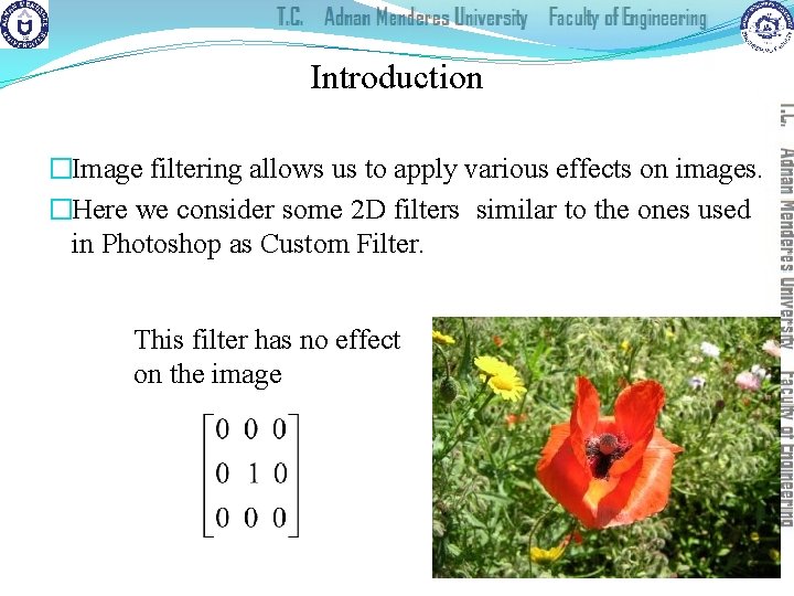
Introduction �Image filtering allows us to apply various effects on images. �Here we consider some 2 D filters similar to the ones used in Photoshop as Custom Filter. This filter has no effect on the image

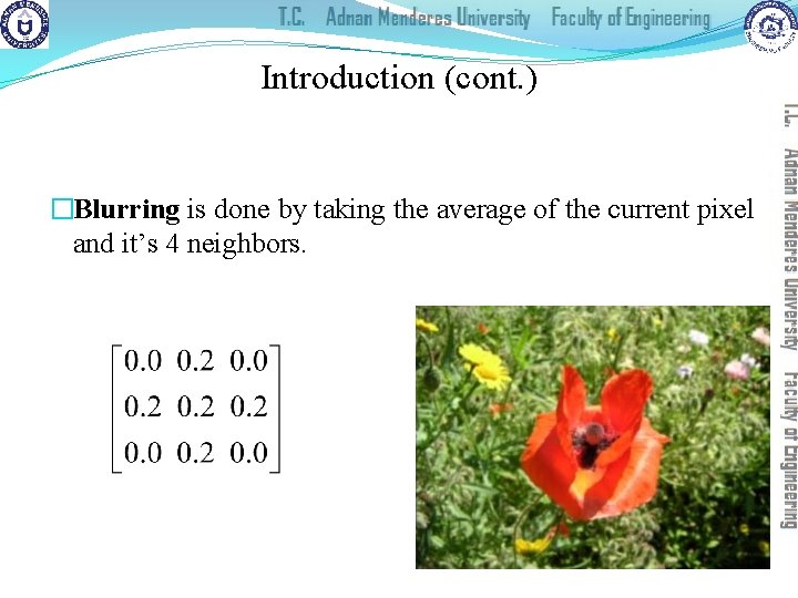
Introduction (cont. ) �Blurring is done by taking the average of the current pixel and it’s 4 neighbors.

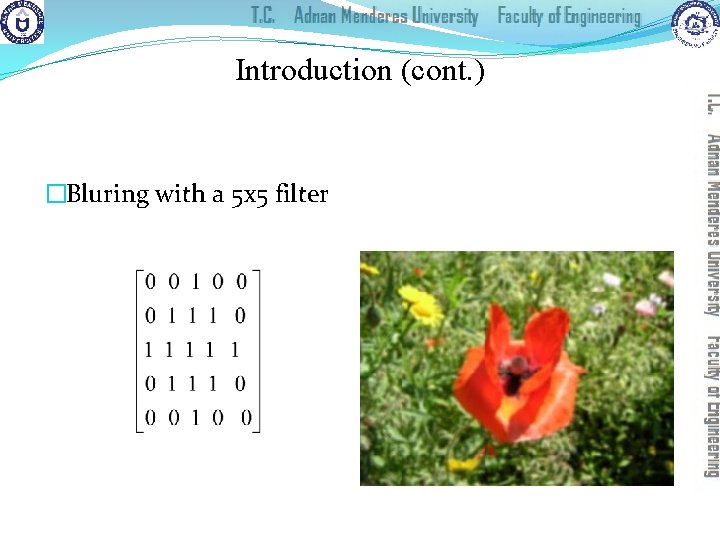
Introduction (cont. ) �Bluring with a 5 x 5 filter

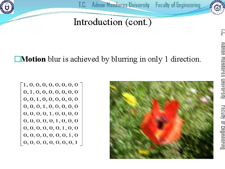
Introduction (cont. ) �Motion blur is achieved by blurring in only 1 direction. +

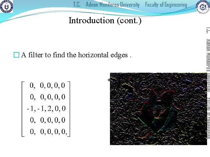
Introduction (cont. ) � A filter to find the horizontal edges. +

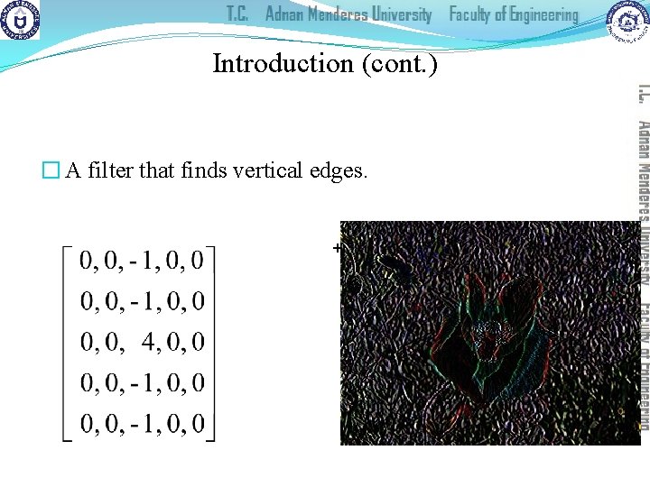
Introduction (cont. ) � A filter that finds vertical edges. +

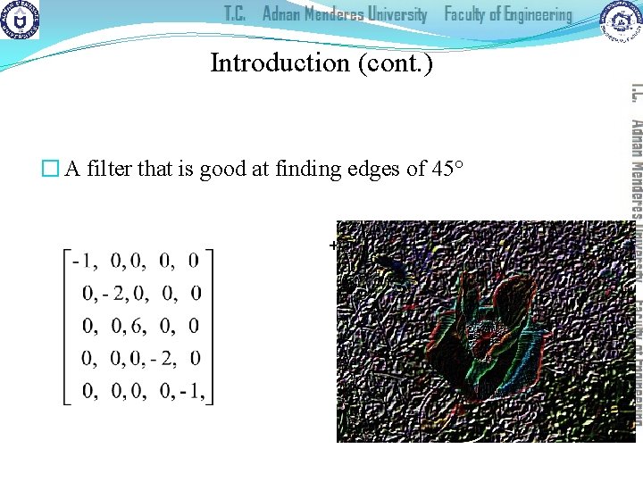
Introduction (cont. ) � A filter that is good at finding edges of 45° +

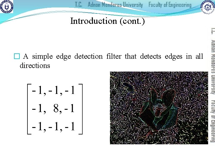
Introduction (cont. ) � A simple edge detection filter that detects edges in all directions +

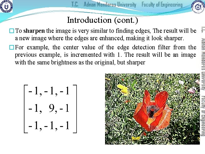
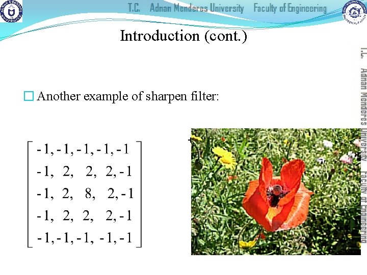
Introduction (cont. ) �To sharpen the image is very similar to finding edges, The result will be a new image where the edges are enhanced, making it look sharper. �For example, the center value of the edge detection filter from the previous example, is incremented with 1. The result will be an image with the same brightness as the original, but sharper +

Introduction (cont. ) � Another example of sharpen filter: +

What is edge detection? § Edge detection is a fundamental image processing operation used in many computer vision solutions. § Goal of edge detection algorithms: to find the most relevant edges in an image or scene. �These edges should then be connected into meaningful lines and boundaries, resulting in a segmented image containing two or more regions. �Subsequent stages in a machine vision system will use the segmented results for tasks such as object counting, measuring, feature extraction, and classification.

What is edge detection? (cont. ) § Biological vision: there is compelling evidence that the very early stages of the human visual system (HVS) contain edge -sensitive cells that respond strongly (i. e. , exhibit a higher firing rate) when presented with edges of certain intensity and orientation. �Edge detection algorithms attempt to emulate an ability present in the HVS. �Such an ability is, according to many vision theorists, essential to all processing steps that take place afterward in the HVS.

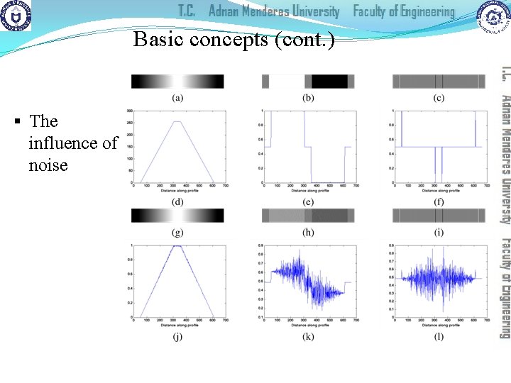
What is edge detection? (cont. ) § Edge detection is a hard image processing problem. § Most edge detection solutions exhibit limited performance in the presence of images containing real-world scenes. § It is common to precede the edge detection stage with preprocessing operations such as noise reduction and illumination correction

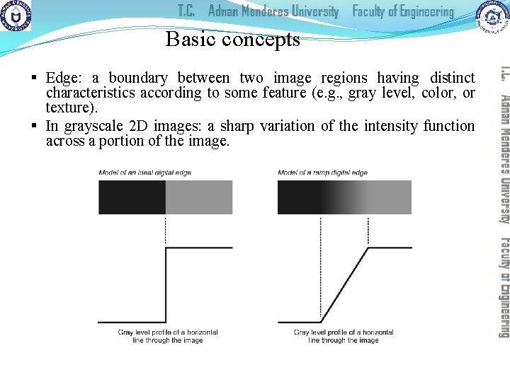
Basic concepts § Edge: a boundary between two image regions having distinct characteristics according to some feature (e. g. , gray level, color, or texture). § In grayscale 2 D images: a sharp variation of the intensity function across a portion of the image.

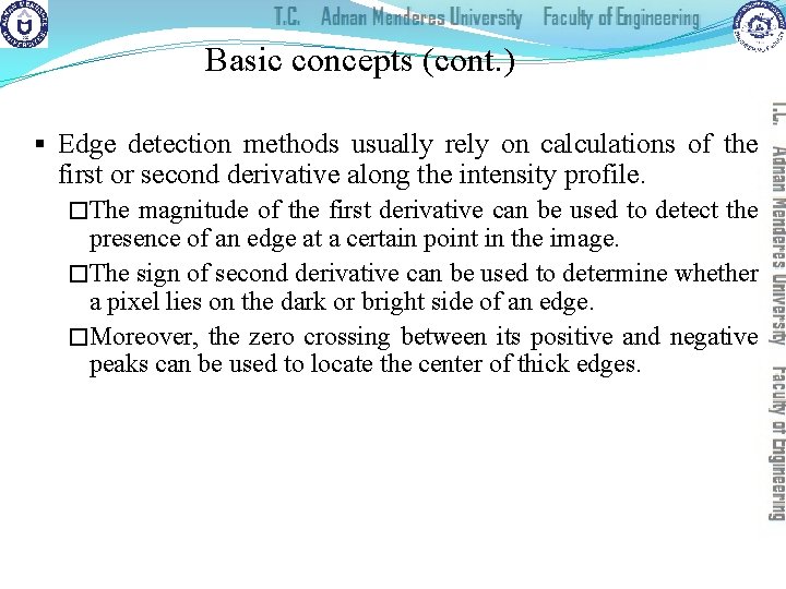
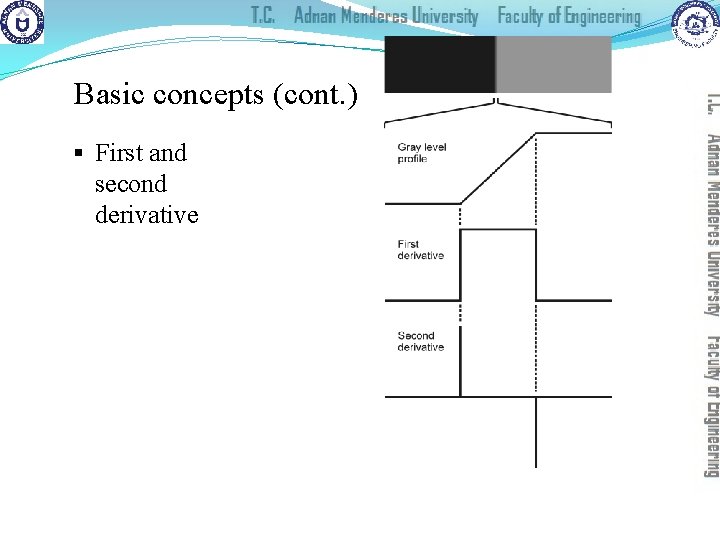
Basic concepts (cont. ) § Edge detection methods usually rely on calculations of the first or second derivative along the intensity profile. �The magnitude of the first derivative can be used to detect the presence of an edge at a certain point in the image. �The sign of second derivative can be used to determine whether a pixel lies on the dark or bright side of an edge. �Moreover, the zero crossing between its positive and negative peaks can be used to locate the center of thick edges.

Basic concepts (cont. ) § First and second derivative

Basic concepts (cont. ) § The influence of noise

Basic concepts (cont. ) § The process of edge detection consists of three main steps: �Noise reduction �Detection of edge points �Edge localization § In MATLAB: edge

Background: Derivatives (remember? ) § First-order derivative § Second-order derivative

Characteristics of First and Second Order Derivatives § First-order derivatives generally produce thicker edges in image § Second-order derivatives have a stronger response to fine detail, such as thin lines, isolated points, and noise § Second-order derivatives produce a double-edge response(negative to positive or positive to negative at ramp and step transition in intensity § The sign of the second derivative can be used to determine whether a transition into an edge is from light to dark or dark to light

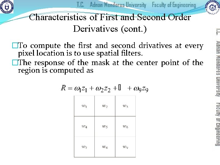
Characteristics of First and Second Order Derivatives (cont. ) �To compute the first and second drivatives at every pixel location is to use spatial filters. �The response of the mask at the center point of the region is computed as

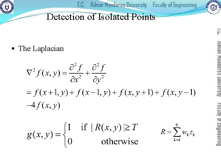
Detection of Isolated Points § The Laplacian

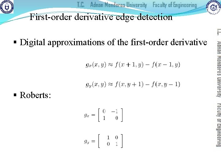
First-order derivative edge detection § Digital approximations of the first-order derivative § Roberts:

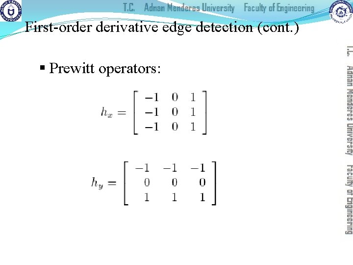
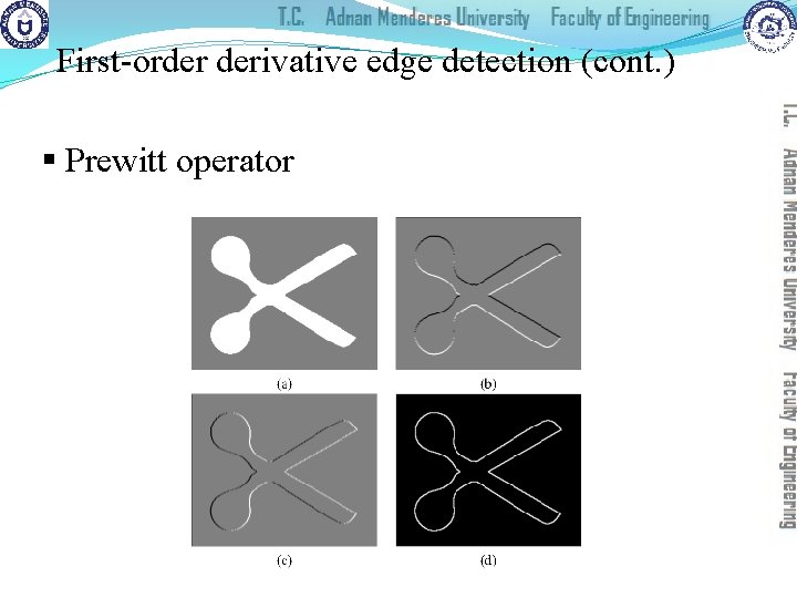
First-order derivative edge detection (cont. ) § Prewitt operators:

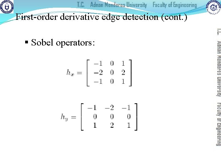
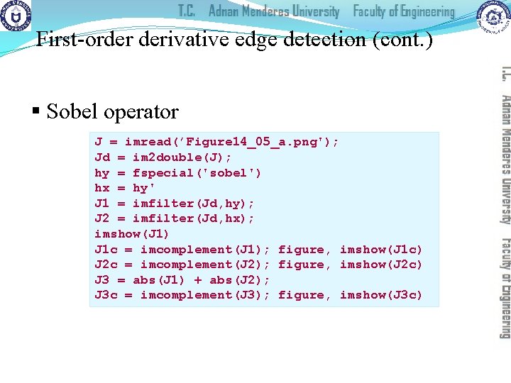
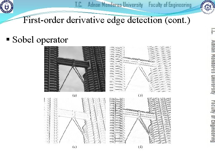
First-order derivative edge detection (cont. ) § Sobel operators:

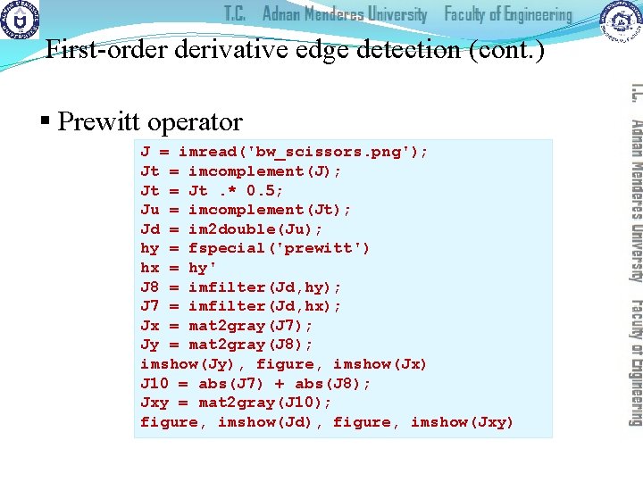
First-order derivative edge detection (cont. ) § Prewitt operator J = imread('bw_scissors. png'); Jt = imcomplement(J); Jt = Jt. * 0. 5; Ju = imcomplement(Jt); Jd = im 2 double(Ju); hy = fspecial('prewitt') hx = hy' J 8 = imfilter(Jd, hy); J 7 = imfilter(Jd, hx); Jx = mat 2 gray(J 7); Jy = mat 2 gray(J 8); imshow(Jy), figure, imshow(Jx) J 10 = abs(J 7) + abs(J 8); Jxy = mat 2 gray(J 10); figure, imshow(Jd), figure, imshow(Jxy)

First-order derivative edge detection (cont. ) § Prewitt operator

First-order derivative edge detection (cont. ) § Sobel operator J = imread(’Figure 14_05_a. png'); Jd = im 2 double(J); hy = fspecial('sobel') hx = hy' J 1 = imfilter(Jd, hy); J 2 = imfilter(Jd, hx); imshow(J 1) J 1 c = imcomplement(J 1); figure, imshow(J 1 c) J 2 c = imcomplement(J 2); figure, imshow(J 2 c) J 3 = abs(J 1) + abs(J 2); J 3 c = imcomplement(J 3); figure, imshow(J 3 c)

First-order derivative edge detection (cont. ) § Sobel operator

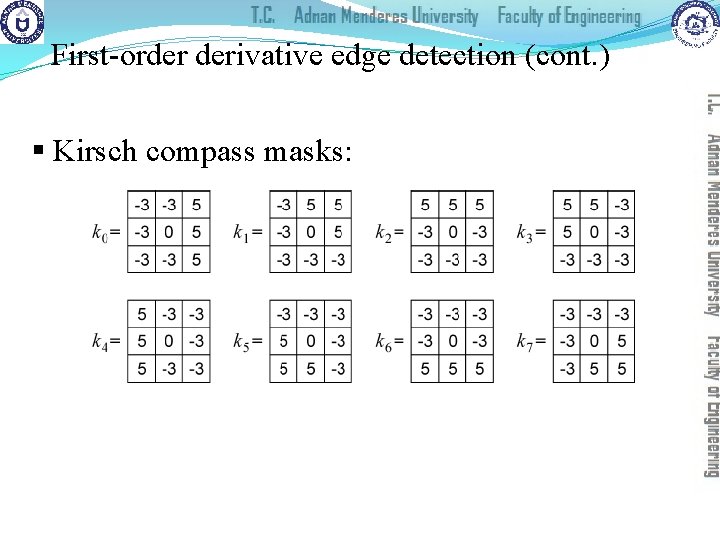
First-order derivative edge detection (cont. ) § Kirsch compass masks:

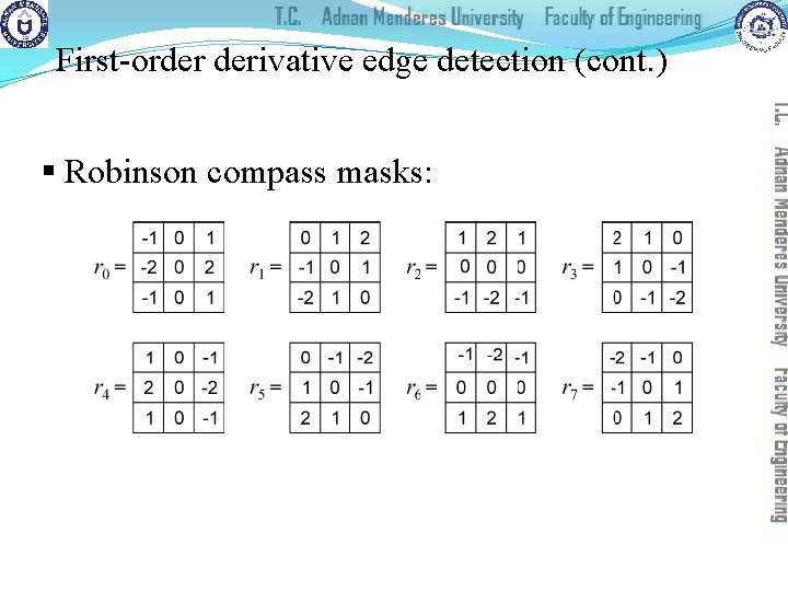
First-order derivative edge detection (cont. ) § Robinson compass masks:

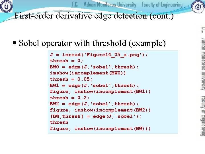
First-order derivative edge detection (cont. ) § Sobel operator with threshold (example) J = imread('Figure 14_05_a. png'); thresh = 0; BW 0 = edge(J, 'sobel', thresh); imshow(imcomplement(BW 0)) thresh = 0. 05; BW 1 = edge(J, 'sobel', thresh); figure, imshow(imcomplement(BW 1)) thresh = 0. 2; BW 2 = edge(J, 'sobel', thresh); figure, imshow(imcomplement(BW 2)) [BW, thresh] = edge(J, 'sobel'); thresh figure, imshow(imcomplement(BW)))

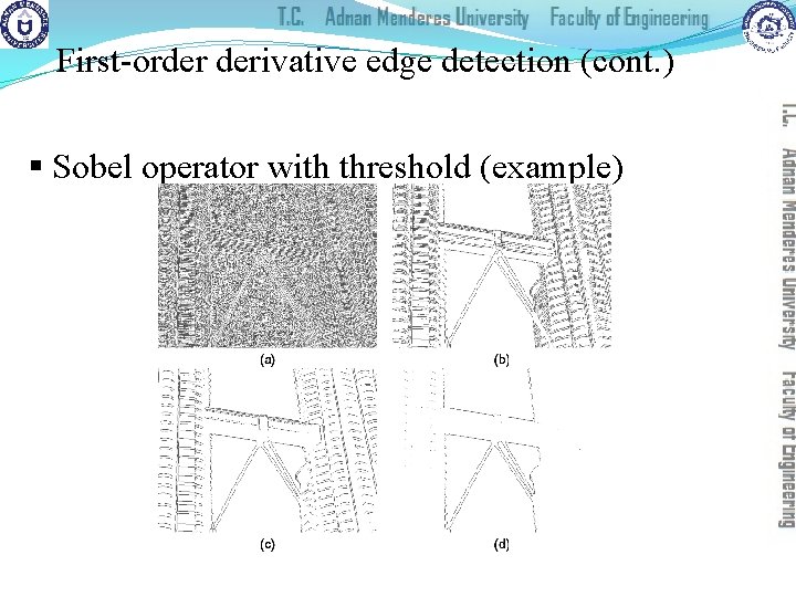
First-order derivative edge detection (cont. ) § Sobel operator with threshold (example)

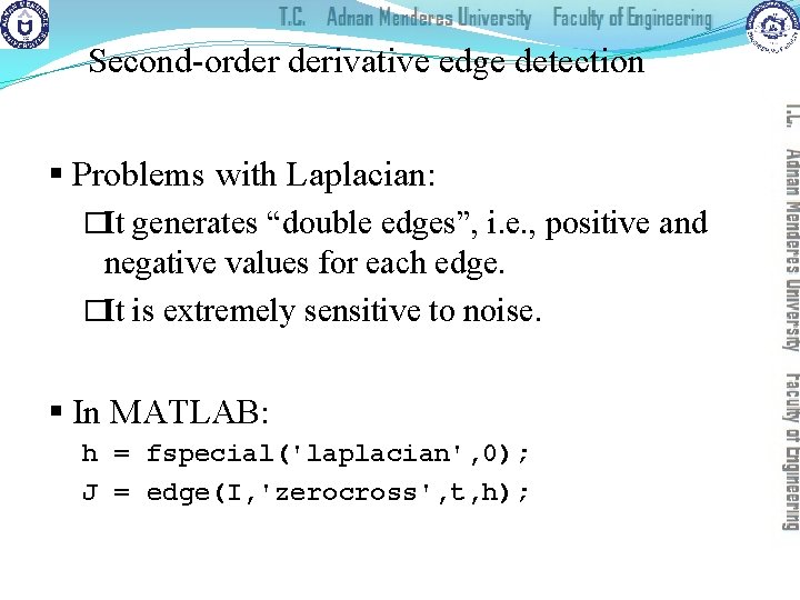
Second-order derivative edge detection § Problems with Laplacian: �It generates “double edges”, i. e. , positive and negative values for each edge. �It is extremely sensitive to noise. § In MATLAB: h = fspecial('laplacian', 0); J = edge(I, 'zerocross', t, h);

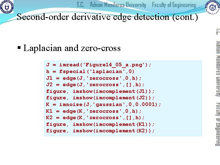
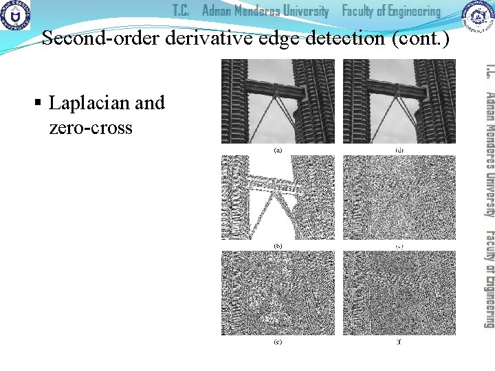
Second-order derivative edge detection (cont. ) § Laplacian and zero-cross J = imread('Figure 14_05_a. png'); h = fspecial('laplacian', 0) J 1 = edge(J, 'zerocross', 0, h); J 2 = edge(J, 'zerocross', [], h); figure, imshow(imcomplement(J 1)); figure, imshow(imcomplement(J 2)); K = imnoise(J, 'gaussian', 0, 0. 0001); K 1 = edge(K, 'zerocross', 0, h); K 2 = edge(K, 'zerocross', [], h); figure, imshow(imcomplement(K 1)); figure, imshow(imcomplement(K 2));

Second-order derivative edge detection (cont. ) § Laplacian and zero-cross

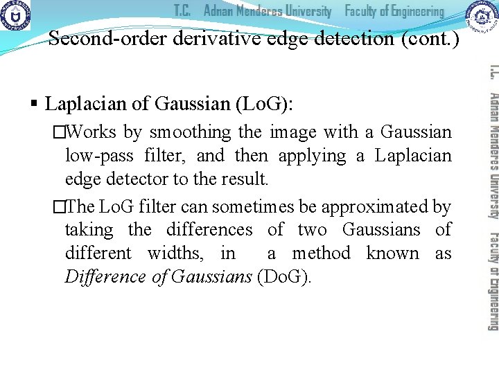
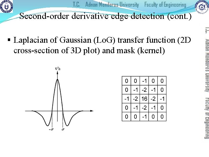
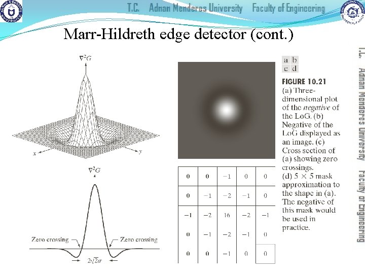
Second-order derivative edge detection (cont. ) § Laplacian of Gaussian (Lo. G): �Works by smoothing the image with a Gaussian low-pass filter, and then applying a Laplacian edge detector to the result. �The Lo. G filter can sometimes be approximated by taking the differences of two Gaussians of different widths, in a method known as Difference of Gaussians (Do. G).

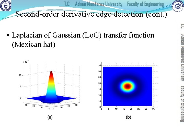
Second-order derivative edge detection (cont. ) § Laplacian of Gaussian (Lo. G) transfer function (Mexican hat)

Second-order derivative edge detection (cont. ) § Laplacian of Gaussian (Lo. G) transfer function (2 D cross-section of 3 D plot) and mask (kernel)

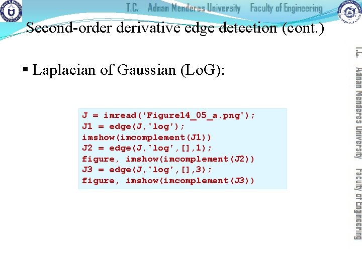
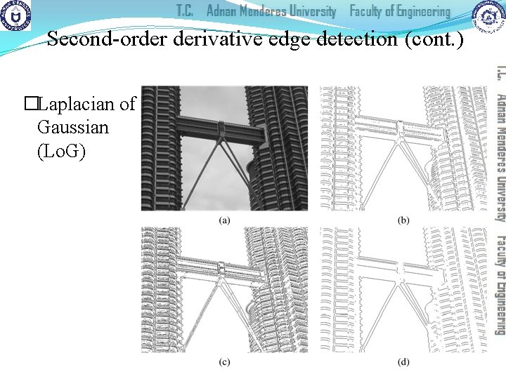
Second-order derivative edge detection (cont. ) § Laplacian of Gaussian (Lo. G): J = imread('Figure 14_05_a. png'); J 1 = edge(J, 'log'); imshow(imcomplement(J 1)) J 2 = edge(J, 'log', [], 1); figure, imshow(imcomplement(J 2)) J 3 = edge(J, 'log', [], 3); figure, imshow(imcomplement(J 3))

Second-order derivative edge detection (cont. ) �Laplacian of Gaussian (Lo. G)

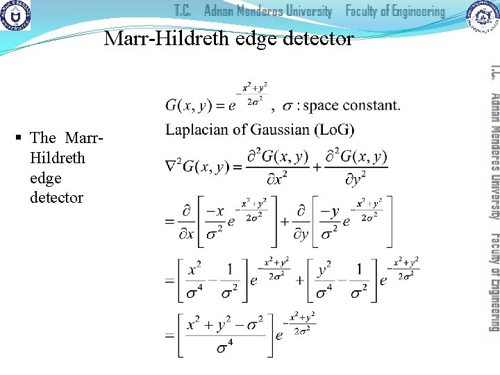
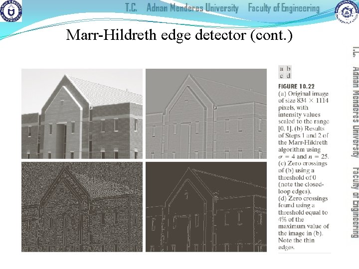
Marr-Hildreth edge detector § The Marr. Hildreth edge detector

Marr-Hildreth edge detector (cont. )

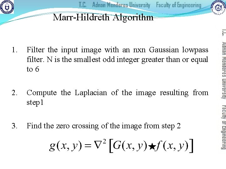
Marr-Hildreth Algorithm 1. Filter the input image with an nxn Gaussian lowpass filter. N is the smallest odd integer greater than or equal to 6 2. Compute the Laplacian of the image resulting from step 1 3. Find the zero crossing of the image from step 2

Marr-Hildreth edge detector (cont. )

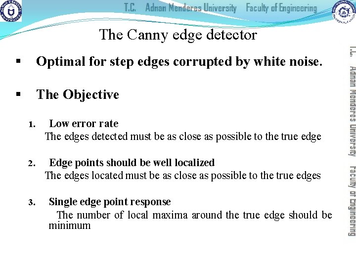
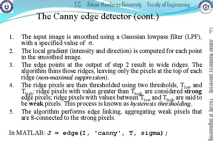
The Canny edge detector § Optimal for step edges corrupted by white noise. § The Objective 1. Low error rate The edges detected must be as close as possible to the true edge 2. Edge points should be well localized The edges located must be as close as possible to the true edges 3. Single edge point response The number of local maxima around the true edge should be minimum

The Canny edge detector (cont. ) 1. 2. 3. 4. 5. The input image is smoothed using a Gaussian lowpass filter (LPF), with a specified value of σ. The local gradient (intensity and direction) is computed for each point in the smoothed image. The edge points at the output of step 2 result in wide ridges. The algorithm thins those ridges, leaving only the pixels at the top of each ridge (non-maximal suppression). The ridge pixels are then thresholded using two thresholds, Tlow and Thigh: ridge pixels with value greater than Thigh are considered strong edge pixels; ridge pixels with values between Tlow and Thigh are said to be weak pixels. This process is known as hysteresis thresholding. The algorithm performs edge linking, aggregating weak pixels that are 8 -connected to the strong pixels. In MATLAB: J = edge(I, 'canny', T, sigma);

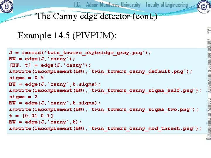
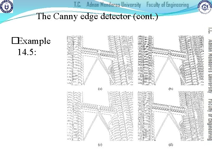
The Canny edge detector (cont. ) Example 14. 5 (PIVPUM): J = imread('twin_towers_skybridge_gray. png'); BW = edge(J, 'canny'); [BW, t] = edge(J, 'canny'); imwrite(imcomplement(BW), 'twin_towers_canny_default. png'); sigma = 0. 5 BW = edge(J, 'canny', t, sigma); imwrite(imcomplement(BW), 'twin_towers_canny_sigma_half. png'); sigma = 2 BW = edge(J, 'canny', t, sigma); imwrite(imcomplement(BW), 'twin_towers_canny_sigma_two. png'); t = [0. 01 0. 1] BW = edge(J, 'canny', t); imwrite(imcomplement(BW), 'twin_towers_canny_mod_thresh. png');

The Canny edge detector (cont. ) �Example 14. 5:

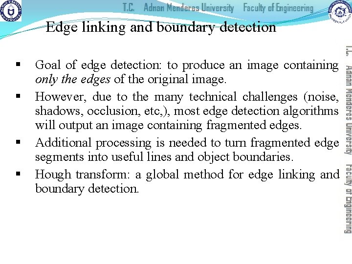
Edge linking and boundary detection § § Goal of edge detection: to produce an image containing only the edges of the original image. However, due to the many technical challenges (noise, shadows, occlusion, etc, ), most edge detection algorithms will output an image containing fragmented edges. Additional processing is needed to turn fragmented edge segments into useful lines and object boundaries. Hough transform: a global method for edge linking and boundary detection.

The Hough transform (cont. ) § A mathematical method designed to find lines in images. �It can be used for linking the results of edge detection, turning potentially sparse, broken, or isolated edges into useful lines that correspond to the actual edges in the image.

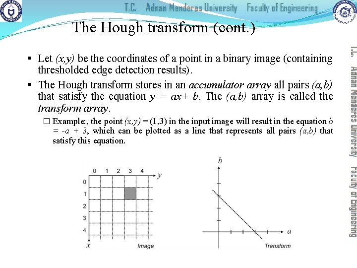
The Hough transform (cont. ) § Let (x, y) be the coordinates of a point in a binary image (containing thresholded edge detection results). § The Hough transform stores in an accumulator array all pairs (a, b) that satisfy the equation y = ax+ b. The (a, b) array is called the transform array. � Example: , the point (x, y) = (1, 3) in the input image will result in the equation b = -a + 3, which can be plotted as a line that represents all pairs (a, b) that satisfy this equation.

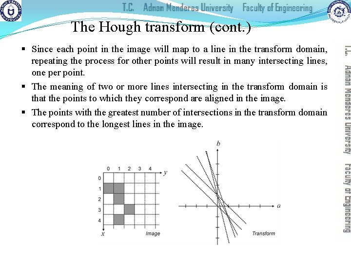
The Hough transform (cont. ) § Since each point in the image will map to a line in the transform domain, repeating the process for other points will result in many intersecting lines, one per point. § The meaning of two or more lines intersecting in the transform domain is that the points to which they correspond are aligned in the image. § The points with the greatest number of intersections in the transform domain correspond to the longest lines in the image.

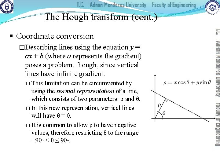
The Hough transform (cont. ) § Coordinate conversion �Describing lines using the equation y = ax + b (where a represents the gradient) poses a problem, though, since vertical lines have infinite gradient. � This limitation can be circumvented by using the normal representation of a line, which consists of two parameters: ρ and θ. � In this new representation, vertical lines will have θ = 0. � It is common to allow ρ to have negative values, therefore restricting θ to the range − 90◦ < θ ≤ 90◦.

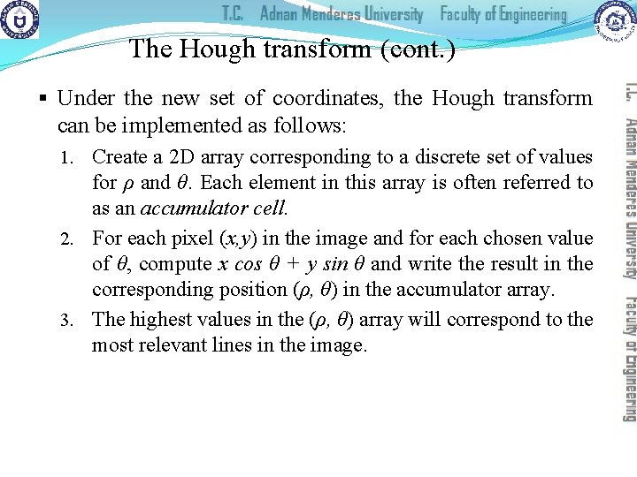
The Hough transform (cont. ) § Under the new set of coordinates, the Hough transform can be implemented as follows: 1. Create a 2 D array corresponding to a discrete set of values for ρ and θ. Each element in this array is often referred to as an accumulator cell. 2. For each pixel (x, y) in the image and for each chosen value of θ, compute x cos θ + y sin θ and write the result in the corresponding position (ρ, θ) in the accumulator array. 3. The highest values in the (ρ, θ) array will correspond to the most relevant lines in the image.

The Hough transform (cont. ) § In MATLAB: �The IPT contains a function for Hough transform calculations, hough, which takes a binary image as an input parameter, and returns the corresponding Hough transform matrix and the arrays of ρ and θ values over which the Hough transform was calculated. �Optionally, the resolution of the discretized 2 D array for both ρ and θ can be specified as additional parameters.

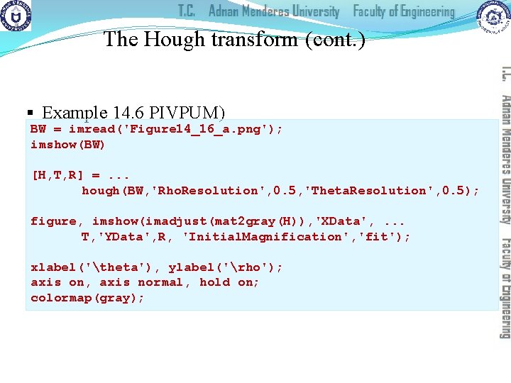
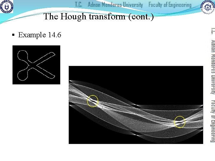
The Hough transform (cont. ) § Example 14. 6 PIVPUM) BW = imread('Figure 14_16_a. png'); imshow(BW) [H, T, R] =. . . hough(BW, 'Rho. Resolution', 0. 5, 'Theta. Resolution', 0. 5); figure, imshow(imadjust(mat 2 gray(H)), 'XData', . . . T, 'YData', R, 'Initial. Magnification', 'fit'); xlabel('theta'), ylabel('rho'); axis on, axis normal, hold on; colormap(gray);

The Hough transform (cont. ) § Example 14. 6

The Hough transform (cont. ) § In MATLAB: �The IPT also includes two useful companion functions for exploring and plotting the results of Hough Transform calculations: identifies the k most salient peaks in the Hough transform results, where k is passed as a parameter. � houghlines: draws the lines associated with the highest peaks on top of the original image. � houghpeaks:

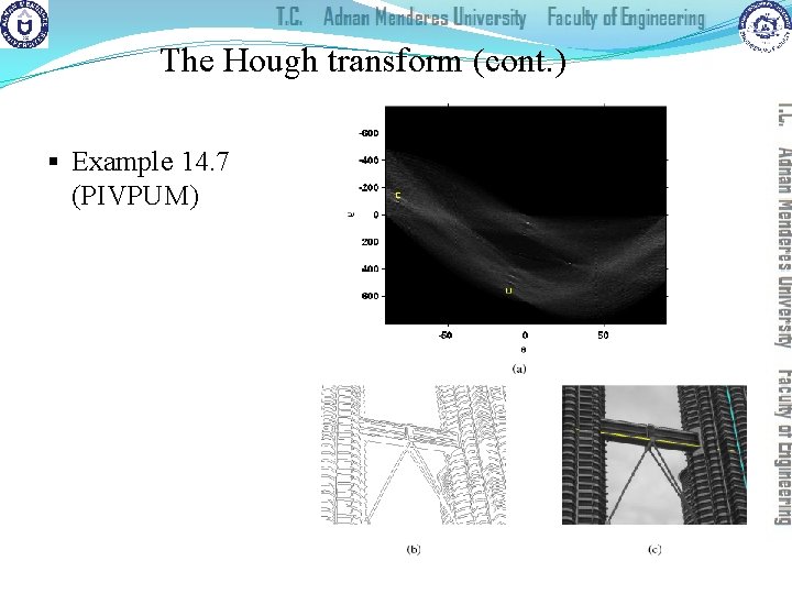
The Hough transform (cont. ) § Example 14. 7 (PIVPUM)

Summary § You should now know �What edge detection is and its importance in computer vision �The main edge detection techniques and how well they work �How you can perform edge detection in MATLAB �What the Hough Transform is and how it can be used to post -process the results of an edge detection algorithm

References § Rafael C. Gonzalez, Richard E. Woods, “Digital Image Processing, 4 th Ed. ”; Pearson, 2018, (DIP) § Rafael C. Gonzalez, Richard E. Woods, Steven L. Eddins, “Digital Image Processing Using MATLAB”; Pearson, 2004, (DIPUM) § Oge Marques, “Practical Image and Video Processing Using MATLAB”; Wiley, 2011, (PIVPUM)