Learning CMPT 310 Simon Fraser University Oliver Schulte
- Slides: 40

Learning CMPT 310 Simon Fraser University Oliver Schulte

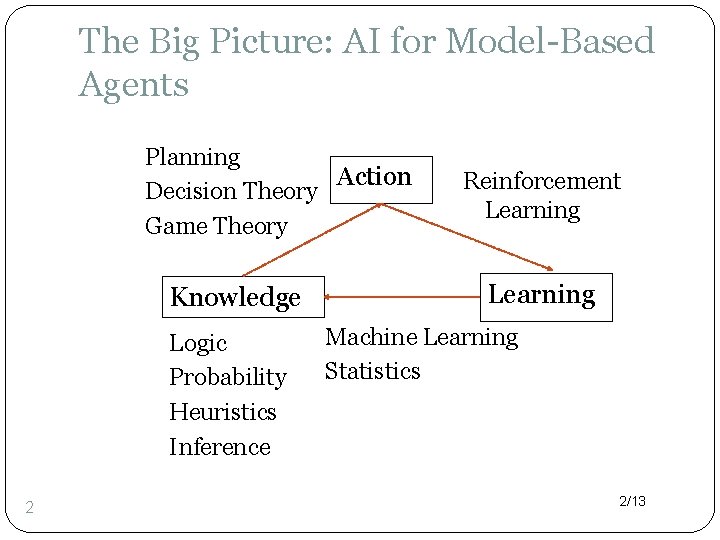
The Big Picture: AI for Model-Based Agents Planning Action Decision Theory Game Theory Knowledge Logic Probability Heuristics Inference 2 Artificial Intelligence a modern approach Reinforcement Learning Machine Learning Statistics 2/13

Motivation �Building a knowledge base is a significant investment of time and resources. �Prone to error, needs debugging. �Alternative approach: Learn rules from examples. �Grand Vision: Start with “seed rules” from expert, use examples to expand refine. 3/13

Overview �Many learning models exist. �Will consider two representative ones that are widely used in AI. �Learning Bayesian network parameters. �Learning a decision tree classifier. 4/13

Examples �Program By Example Excel Flash Fill �Kaggle Data Science Competitions 5/13

Learning Bayesian Networks 6/13

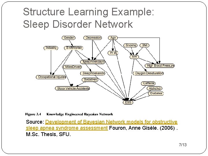
Structure Learning Example: Sleep Disorder Network Source: Development of Bayesian Network models for obstructive sleep apnea syndrome assessment Fouron, Anne Gisèle. (2006). M. Sc. Thesis, SFU. 7/13

Parameter Learning Common Approach �Expert specifies Bayesian network structure (nodes and links). �Program fills in parameters (conditional probabilities). 8/13

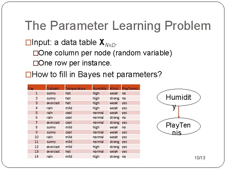
The Parameter Learning Problem �Input: a data table XNx. D. �One column per node (random variable) �One row per instance. �How to fill in Bayes net parameters? Day 1 2 3 4 5 6 7 8 9 10 11 12 13 14 Outlook sunny overcast rain overcast sunny rain sunny overcast rain Temperature hot hot mild cool mild hot mild Humidity high normal normal high Wind weak strong weak weak strong weak strong Play. Tennis no no yes yes yes no Humidit y Play. Ten nis 10/13

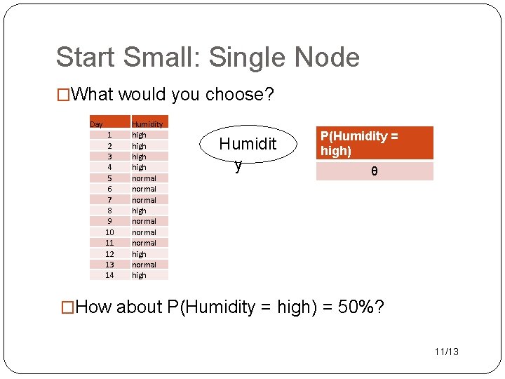
Start Small: Single Node �What would you choose? Day 1 2 3 4 5 6 7 8 9 10 11 12 13 14 Humidity high normal normal high Humidit y P(Humidity = high) θ �How about P(Humidity = high) = 50%? 11/13

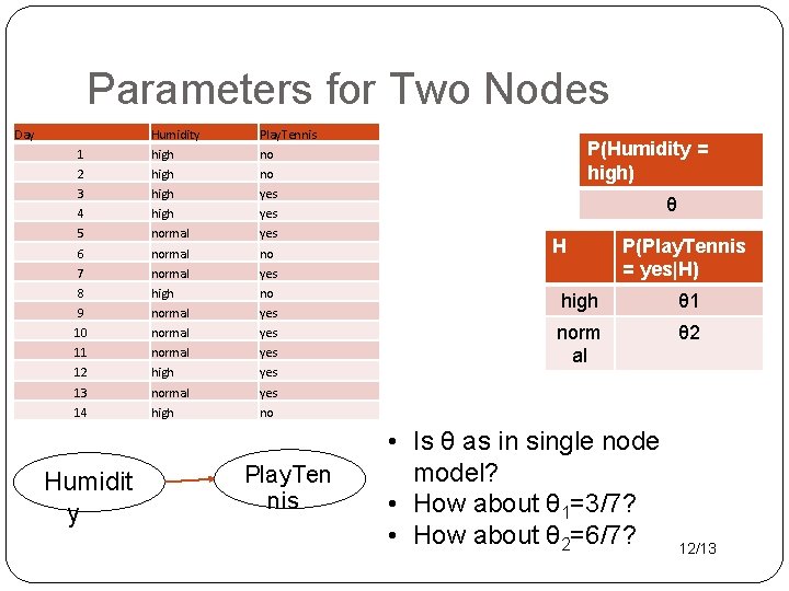
Parameters for Two Nodes Day Humidity Play. Tennis 1 high no 2 high no 3 high yes 4 high yes 5 normal yes 6 normal no 7 normal yes 8 high no 9 normal yes 10 normal yes 11 normal yes 12 high yes 13 normal yes 14 high no Humidit y Play. Ten nis P(Humidity = high) θ H P(Play. Tennis = yes|H) high θ 1 norm al θ 2 • Is θ as in single node model? • How about θ 1=3/7? • How about θ 2=6/7? 12/13

Maximum Likelihood Estimation 13/13

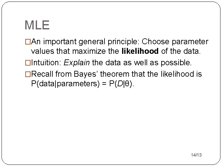
MLE �An important general principle: Choose parameter values that maximize the likelihood of the data. �Intuition: Explain the data as well as possible. �Recall from Bayes’ theorem that the likelihood is P(data|parameters) = P(D|θ). 14/13

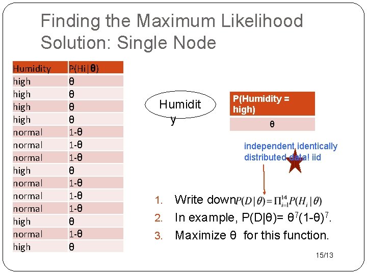
Finding the Maximum Likelihood Solution: Single Node Humidity high normal normal high P(Hi|θ) θ θ 1 -θ 1 -θ 1 -θ θ Humidit y P(Humidity = high) θ independent identically distributed data! iid Write down 2. In example, P(D|θ)= θ 7(1 -θ)7. 3. Maximize θ for this function. 1. 15/13

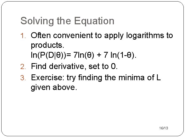
Solving the Equation 1. Often convenient to apply logarithms to products. ln(P(D|θ))= 7 ln(θ) + 7 ln(1 -θ). 2. Find derivative, set to 0. 3. Exercise: try finding the minima of L given above. 16/13

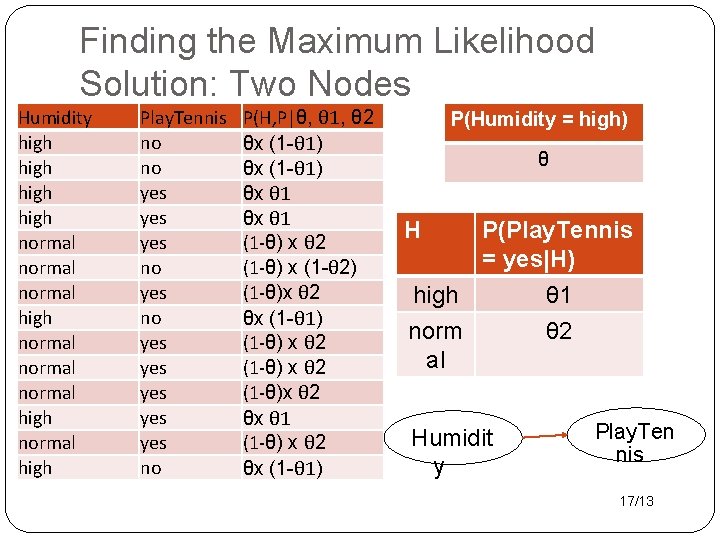
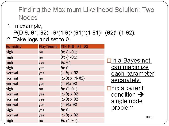
Finding the Maximum Likelihood Solution: Two Nodes Humidity high normal normal high Play. Tennis no no yes yes yes no P(H, P|θ, θ 1, θ 2 θx (1 -θ 1) θx θ 1 (1 -θ) x θ 2 (1 -θ) x (1 -θ 2) (1 -θ)x θ 2 θx (1 -θ 1) (1 -θ) x θ 2 (1 -θ)x θ 2 θx θ 1 (1 -θ) x θ 2 θx (1 -θ 1) P(Humidity = high) θ H P(Play. Tennis = yes|H) high norm al Humidit y θ 1 θ 2 Play. Ten nis 17/13

Finding the Maximum Likelihood Solution: Two Nodes 1. In example, P(D|θ, θ 1, θ 2)= θ 7(1 -θ)7 (θ 1)3(1 -θ 1)4 (θ 2)6 (1 -θ 2). 2. Take logs and set to 0. Humidity high normal normal high Play. Tennis no no yes yes yes no P(H, P|θ, θ 1, θ 2 θx (1 -θ 1) θx θ 1 (1 -θ) x θ 2 (1 -θ) x (1 -θ 2) (1 -θ)x θ 2 θx (1 -θ 1) (1 -θ) x θ 2 (1 -θ)x θ 2 θx θ 1 (1 -θ) x θ 2 θx (1 -θ 1) �In a Bayes net, can maximize each parameter separately. �Fix a parent condition single node problem. 18/13

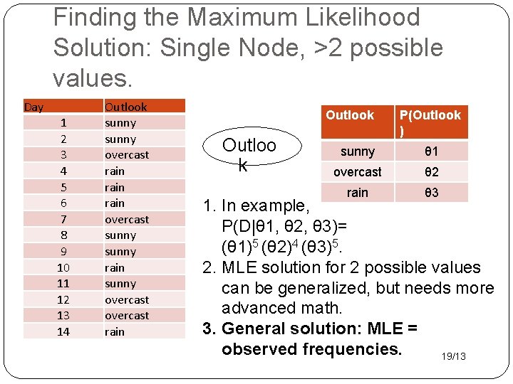
Finding the Maximum Likelihood Solution: Single Node, >2 possible values. Day 1 2 3 4 5 6 7 8 9 10 11 12 13 14 Outlook sunny overcast rain overcast sunny rain sunny overcast rain Outlook Outloo k P(Outlook ) sunny θ 1 overcast θ 2 rain θ 3 1. In example, P(D|θ 1, θ 2, θ 3)= (θ 1)5 (θ 2)4 (θ 3)5. 2. MLE solution for 2 possible values can be generalized, but needs more advanced math. 3. General solution: MLE = observed frequencies. 19/13

Decision Tree Classifiers

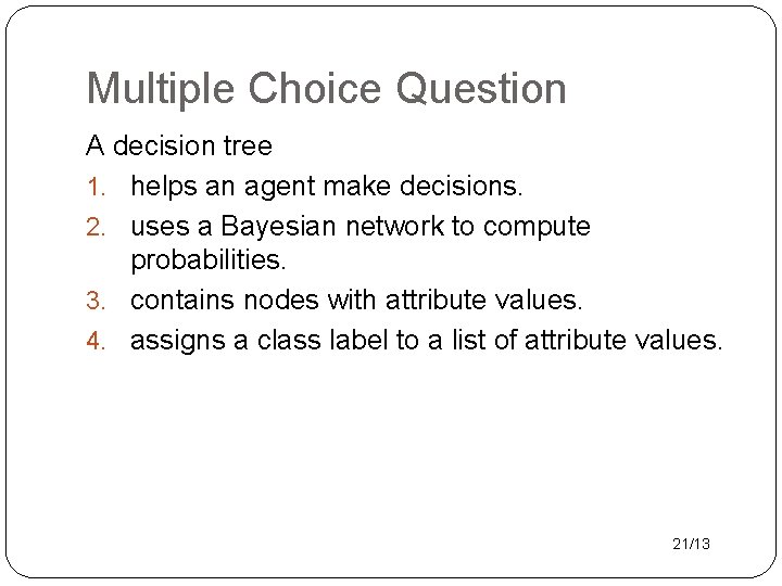
Multiple Choice Question A decision tree 1. helps an agent make decisions. 2. uses a Bayesian network to compute probabilities. 3. contains nodes with attribute values. 4. assigns a class label to a list of attribute values. 21/13

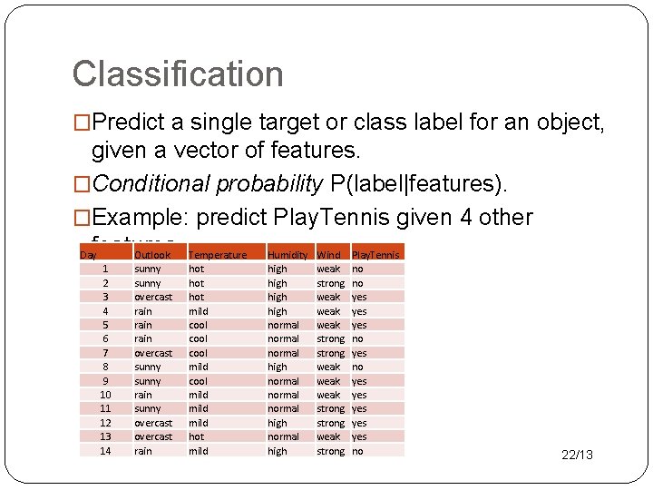
Classification �Predict a single target or class label for an object, given a vector of features. �Conditional probability P(label|features). �Example: predict Play. Tennis given 4 other Dayfeatures. Outlook Temperature Humidity Wind Play. Tennis 1 2 3 4 5 6 7 8 9 10 11 12 13 14 sunny overcast rain overcast sunny rain sunny overcast rain hot hot mild cool mild hot mild high normal normal high weak strong weak weak strong weak strong no no yes yes yes no 22/13

Decision Tree �Popular type of classifier. Easy to visualize. �Especially for discrete values, but also for continuous. �Learning: Information Theory. 23/13

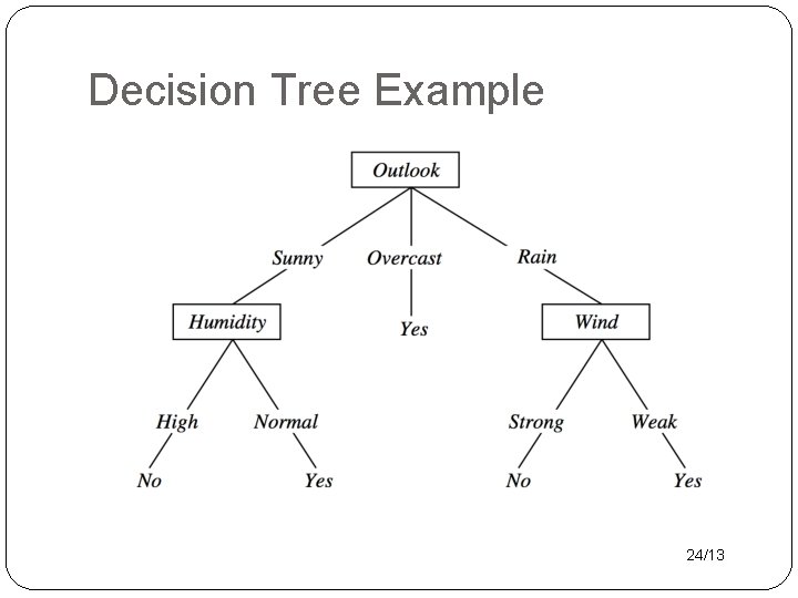
Decision Tree Example 24/13

Exercise Find a decision tree to represent �A OR B, A AND B. �(A AND B) OR (C AND not. D AND E). 25/13

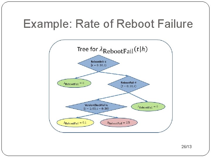
Example: Rate of Reboot Failure 26/13

Big Decision Tree for NHL Goal Scoring 27/13

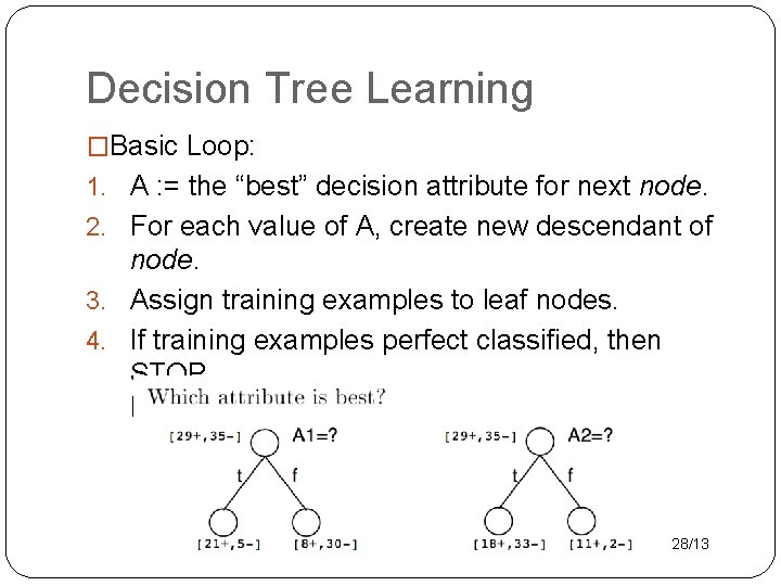
Decision Tree Learning �Basic Loop: 1. A : = the “best” decision attribute for next node. 2. For each value of A, create new descendant of node. 3. Assign training examples to leaf nodes. 4. If training examples perfect classified, then STOP. Else iterate over new leaf nodes. 28/13

Entropy

Multiple Choice Question Entropy 1. measures the amount of uncertainty in a probability distribution. 2. is a concept from relativity theory in physics. 3. refers to the flexibility of an intelligent agent. 4. is maximized by the ID 3 algorithm. 30/13

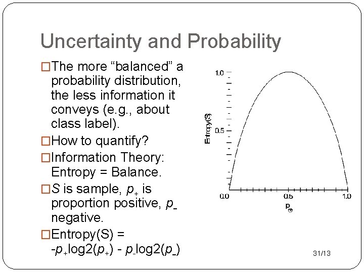
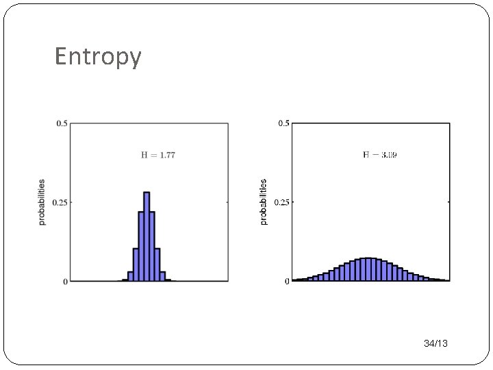
Uncertainty and Probability �The more “balanced” a probability distribution, the less information it conveys (e. g. , about class label). �How to quantify? �Information Theory: Entropy = Balance. �S is sample, p+ is proportion positive, pnegative. �Entropy(S) = -p+log 2(p+) - p-log 2(p-) 31/13

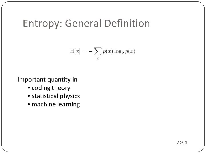
Entropy: General Definition Important quantity in • coding theory • statistical physics • machine learning 32/13

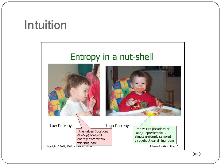
Intuition 33/13

Entropy 34/13

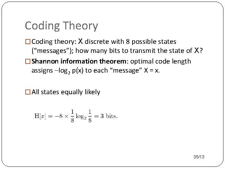
Coding Theory � Coding theory: X discrete with 8 possible states (“messages”); how many bits to transmit the state of X? � Shannon information theorem: optimal code length assigns –log 2 p(x) to each “message” X = x. � All states equally likely 35/13

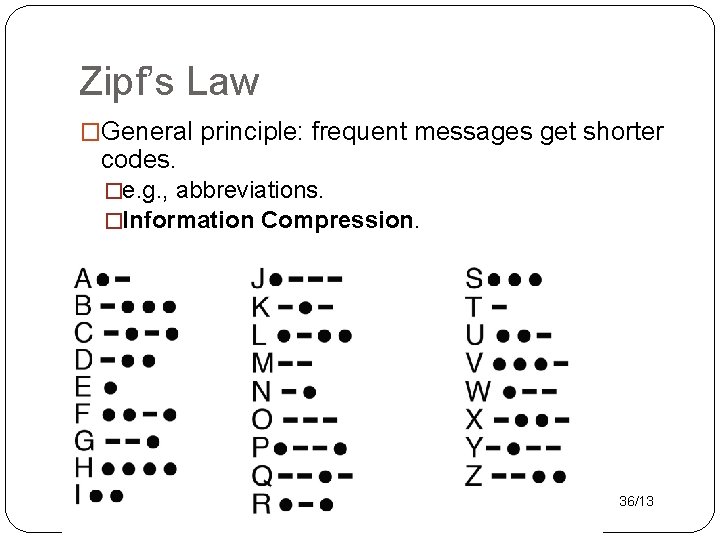
Zipf’s Law �General principle: frequent messages get shorter codes. �e. g. , abbreviations. �Information Compression. 36/13

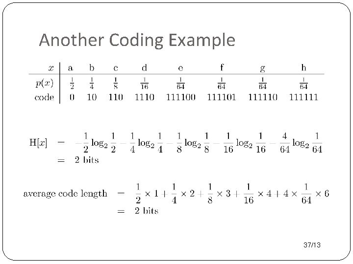
Another Coding Example 37/13

Information Gain ID 3 Decision Tree Learning

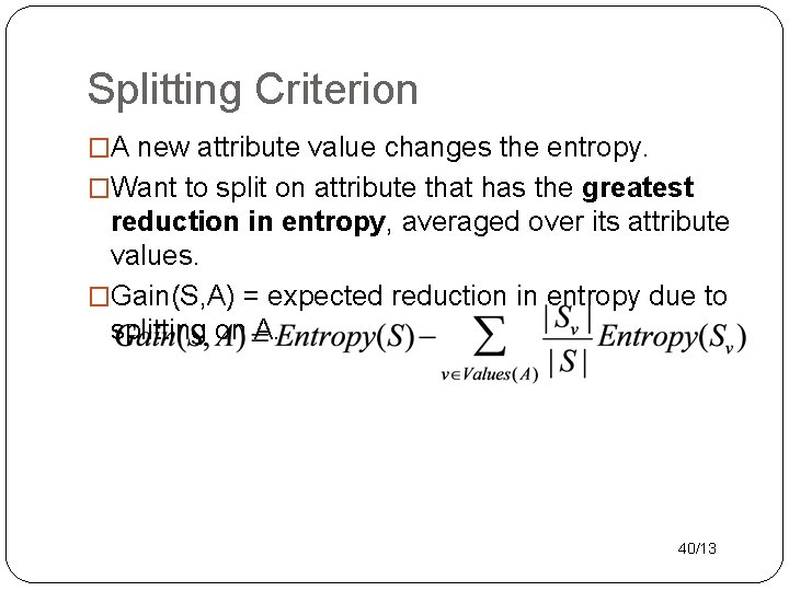
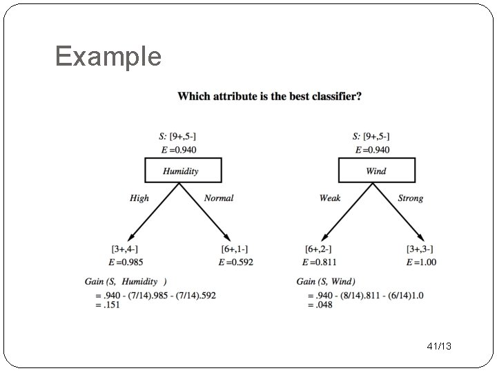
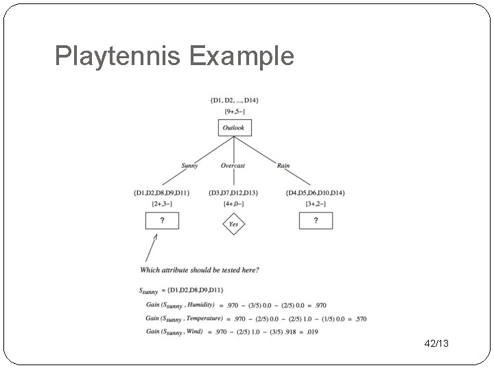
Splitting Criterion �A new attribute value changes the entropy. �Want to split on attribute that has the greatest reduction in entropy, averaged over its attribute values. �Gain(S, A) = expected reduction in entropy due to splitting on A. 40/13

Example 41/13

Playtennis Example 42/13