594 Chapter 11 Orthogonal Functions and Fourier Series
")

 inner product (pp.")
![597 11. 1. 2 定義 (1) inner product on an interval [a, b] (f](https://slidetodoc.com/presentation_image_h2/dc4894f5d5e108523f879525faf3cf26/image-4.jpg "597 11. 1. 2 定義 (1) inner product on an interval [a, b] (f")
 (f 1, f 2) = (f 2, f 1)*")
![599 (2) orthogonal on an interval [a, b] (f 1, f 2 為 real](https://slidetodoc.com/presentation_image_h2/dc4894f5d5e108523f879525faf3cf26/image-6.jpg "599 (2) orthogonal on an interval [a, b] (f 1, f 2 為 real")
 orthogonal set 有一組 functions 0(x), 1(x), 2(x), 3(x), ………. . 若 for")
 Show that the set {1, cosx, cos 2 x,")
 square norm 比較: discrete case (5) norm (6) orthonormal set 對一個 orthogonal")
 Calculate the norms of {1, cosx, cos 2")
 normalize 將 norm 變為 1 (x) 注意,此時 可藉由 normalization, 將 orthogonal set")
![605 (8) complete 若在 interval [a, b] 之間,任何一個 function f(x) 都可以表 示成 0(x), 1(x),](https://slidetodoc.com/presentation_image_h2/dc4894f5d5e108523f879525faf3cf26/image-12.jpg "605 (8) complete 若在 interval [a, b] 之間,任何一個 function f(x) 都可以表 示成 0(x), 1(x),")
(10) 若 0(x), 1(x), 2(x), 3(x), ………. . 為complete 可將 f(x) 表示成 被稱作")
, 1(x), 2(x), 3(x), ………. . 為 orthonormal 607")
 inner product with weight function")
 norm 的定義改成 (11 -4) orthonormal 的定義改成 for m n (11 -5)")
 orthogonal series expansion of f(x) 以及 generalize Fourier series 的算法改成")
 cos(a + b) cosa cosb − sina sinb")
 cos 2 a − sin 2 a or 1 − 2")


 名詞 trigonometric function (page 620) Fourier series (trigonometric series) (page 624) Fourier")
 是個常用字,以 Hz (每秒多少個週期)為單位 說話聲音: 100~1200 Hz 人耳可聽見的聲音: 20~20000 Hz 廣播 (AM):")

 Cosine VS. Sine (when h k) when (h = k)")
 Cosine VS. Cosine, k h when h k (5) Sine VS. Sine,")


 625")

 f 1(x 0) =")
 Example 1 的例子 Fig. 11 -2 -1 if f(x) is not continuous")


 S 3(x) Fig. 11. 2. 3 (b) S 8(x)")
 S 15(x) Fig. 11. 2. 3 N = 15")
")
 重要名詞: Fourier cosine series, cosine series (page 643) Fourier sine series, sine series")
 = f( x)")
 Sine functions are odd sin(t)")
 The product of two even functions")
 If f(x) is even, then (g) If f(x) is odd, then (Proof):")
 The Fourier series of an")
 The Fourier series of an odd function on the interval (−p, p)")
 Expand f(x) = x, 2 < x <")
 odd function, 使用 sine series Fig. 11. 3.")

 S 1(x) (c) S 3(x) Fig. 11. 3. 6 (b) S 2(x)")
 is defined in the interval")
, f(x) = x 2, 0<x<L (a) in")
 in a sine series 假設 f(x) = f( x) for −L <")
 in a Fourier series interval 仍為 (0, L) 原本 Fourier series 公式 現在")
 = x 2, 0 < x < L 將三個方法的結果畫成圖形 cosine")

 方法的限制 (註:以下的步驟不包含解 homogeneous solution 還是需要用 Section 4")
 假設 particular solution 的型態為 (Step 3) 代回原式,比較係數,將 A 0, An, Bn 解出來")
 (相關物理定理請複習 Section 5. 1) for 1 < t")
 和 Step 1 的結果代入 Therefore, the particular solution is:")
 公式一些地方易記錯 for cosine series and sine")


 Fourier integral: (和 Fourier")
 complex form 或 exponential form of Fourier integral 比較: Fourier integral 原本的定義 666")
 Fourier cosine integral 或 cosine integral 適用情形: (1) even 或 (2) interval: [0,")

 為 absolutely")
 f(x) 為 piecewise continuous (2)")
 Find the Fourier integral representation of f(x) 674")


 Fourier cosine integral 或")
 Fourier sine integral 或 sine integral 類比於 sine series 適用情形: (1) f(x)")
 Represent (a) by a cosine integral (b) by a")
 681")
 Fig. 14. 3. 4 (b)")

 F 5(x) (b) F 20(x) (b = 5) (b")


")
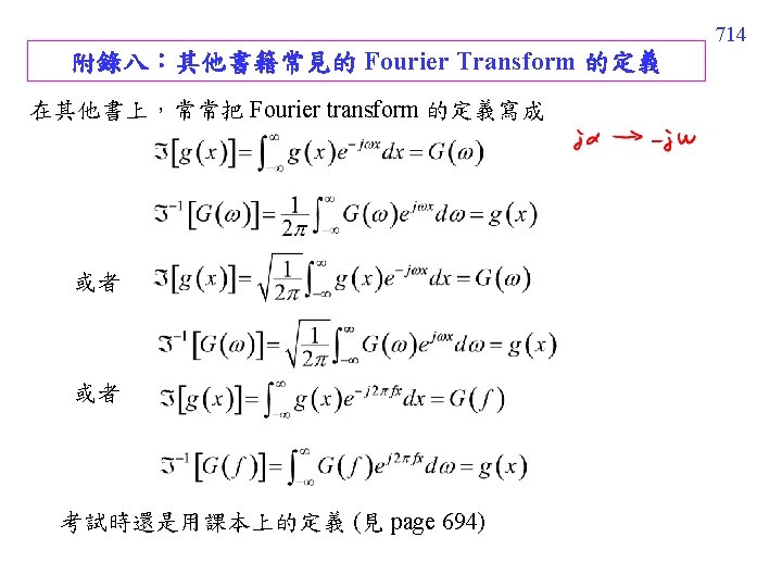
 公式積分的外面,要乘 (Fourier integral) 或 (Complex")

 六大定義 (1) Fourier transform (2) inverse Fourier transform (3) Fourier sine transform")
 微分性質 (7) for Fourier transform (8) (9) for Fourier sine transform 不同")
 Problems with boundary conditions (多練習) (13) 可考慮用 Fourier transform 的情形 (14) 可考慮用 Fourier")


當 f(x) 為 even Fourier transform Fourier cosine")
 Inverse Fourier transform inverse Fourier cosine transform If f(x) is even (由前頁)")
 為 even 的情形。當 f(x) 為")
 Fourier transform 的微分性質做了一些假設: f(x) = 0 when x and")
 Fourier sine transform 的微分性質 (3) Fourier cosine transform 的微分性質 注意: (1) Fourier sine,")

 703 ※ 概念複雜,要特別加強練習 (Condition 1)")

 heat equation: subject to where Step 1 決定針對")

 Step 1 決定針對 y 做 Fourier cosine")

")
 微分公式當中,Fourier cosine transform 和 Fourier")
 在解 partial differential equation 時,往往只針對一個 independent variable 做 Fourier transform, 另一個 independent")

- Slides: 123
594 Chapter 11 Orthogonal Functions and Fourier Series 複習: linear algebra 關於 orthogonal (正交) basis 的介紹 在 linear algebra 當中 (1) inner product (2) orthogonal (3) 若 f 1, f 2, …. , f. N 為 complete orthogonal set, where
例如 在只有三個 entry 的情形下 是一組 complete orthogonal set f 3 f 2 f 1 問題:在 continuous 當中該如何定義 orthogonal? 595
596 Section 11. 1 Orthogonal Functions 11. 1. 1 綱要:熟悉幾個重要定義 (1) inner product (pp. 597) (7) normalize (pp. 604) (2) orthogonal (pp. 599) (8) complete (pp. 605) (3) orthogonal set (pp. 600) (9) orthogonal series expansion (pp. 606) (4) square norm (pp. 602) (10) generalized Fourier series (pp. 606) (5) norm (pp. 602) (11) weight function (pp. 608) With weighting functions, many definition s are changed. 學習方式:(1) 可以多和 linear algebra 當中的定義多比較 (6) orthonormal set (pp. 602) (2) 複習三角函式的公式 (see pp. 611 -612)
597 11. 1. 2 定義 (1) inner product on an interval [a, b] (f 1, f 2 為 real 時) 比較: discrete case 補充:more standard definition for inner product with conjugation
598 Inner product 性質 (a) (f 1, f 2) = (f 2, f 1)* *: conjugation (b) (k f 1, f 2) = k (f 1, f 2), k 為 scalar (或稱為constant) (c) (f, f) = 0 if and only if f = 0, (f, f) > 0 if and only if f 0, (d) (f 1 + f 2 , g) = (f 1, g) + (f 2 , g) discrete case 亦有這些性質
599 (2) orthogonal on an interval [a, b] (f 1, f 2 為 real 時) (more standard definition) 或 比較: discrete case 例子: 當 [a, b] = [-1, 1], 1 和 xk (k 為奇數) 互為 orthogonal 注意:任何 even function 和任何 odd function 在 [-a, a] 之間必為 orthogonal, 包括 Example 1 (text page 426) 的 x 2 和 x 3 在 [-1, 1] 之間也是 orthogonal
600 (3) orthogonal set 有一組 functions 0(x), 1(x), 2(x), 3(x), ………. . 若 for any m n 則 0(x), 1(x), 2(x), 3(x), ………. . 被稱作 orthogonal set on an interval [a, b]
Example 2 (text page 426) Show that the set {1, cosx, cos 2 x, cos 3 x, …. . } is an orthogonal set on the interval [− , ] when one of the functions is 1 when both the two functions are not 1 601
602 (4) square norm 比較: discrete case (5) norm (6) orthonormal set 對一個 orthogonal set, 若更進一步的滿足 for all n 則被稱為 orthonormal set
603 Example 3 (text page 427) Calculate the norms of {1, cosx, cos 2 x, cos 3 x, …. . } 運用三角函式公式 {1, cosx, cos 2 x, cos 3 x, …. . } normalization as a orthonormal set
604 (7) normalize 將 norm 變為 1 (x) 注意,此時 可藉由 normalization, 將 orthogonal set 變成 orthonormal set
605 (8) complete 若在 interval [a, b] 之間,任何一個 function f(x) 都可以表 示成 0(x), 1(x), 2(x), 3(x), ………. . 的 linear combination 則 0(x), 1(x), 2(x), 3(x), ………. . 被稱作 complete 比較:在 linear algebra 當中,對 3 -D vector 而言 e 1 = [1, 0, 0], e 2 = [0, 1, 0], e 3 = [0, 0, 1] 為 complete Any 3 -D vector [a, b, c] can be expressed as ae 1 + be 2 + ce 3
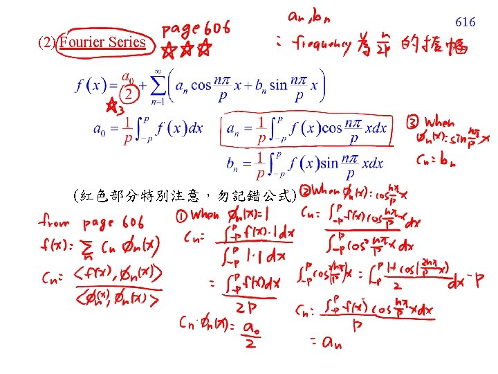
606 (9)(10) 若 0(x), 1(x), 2(x), 3(x), ………. . 為complete 可將 f(x) 表示成 被稱作 (9) orthogonal series expansion 當 0(x), 1(x), 2(x), 3(x), ………. . 不為 orthogonal, cn 不易算 當 0(x), 1(x), 2(x), 3(x), ………. . 為 orthogonal cn 被稱作 (10) generalized Fourier series
當 0(x), 1(x), 2(x), 3(x), ………. . 為 orthonormal 607
608 11. 1. 3 Orthogonal with Weight Function (11) inner product with weight function 其中 w(x) 被稱作 weight function 加上了 weight function 後 (11 -1) orthogonal 的定義改成 for m n (11 -2) square norm 的定義改成
609 (11 -3) norm 的定義改成 (11 -4) orthonormal 的定義改成 for m n (11 -5) normalize 的算法改成
610 (11 -6) orthogonal series expansion of f(x) 以及 generalize Fourier series 的算法改成
611 11. 1. 4 三角函數表 (要複習) cos(a + b) cosa cosb − sina sinb sin(a + b) sina cosb + cosa sinb cos(a − b) cosa cosb + sina sinb sin(a − b) sina cosb − cosa sinb cosa cosb [cos(a + b) + cos(a − b)]/2 sina sinb [cos(a − b) − cos(a + b)]/2 sina cosb [sin(a + b) + sin(a − b)]/2
612 cos(2 a) cos 2 a − sin 2 a or 1 − 2 sin 2 a or 2 cos 2 a − 1 sin(2 a) 2 sin a cos 2 a [cos(2 a) + 1]/2 sin 2 a [1 − cos(2 a)]/2
614 複習: Legendre polynomials 是一種 orthogonal set if m n 其他常用的 orthogonal set Hermite polynomials (with weight function) (補充) Chebyshev polynomials (with weight function) (補充) Cosine series Sine series Fourier series
615 Section 11. 2 Fourier Series 11. 2. 1 綱要 trigonometric functions orthogonal set on the interval of [ p , p] be proved on pages 620~622 週期: 頻率:
617 (3) 名詞 trigonometric function (page 620) Fourier series (trigonometric series) (page 624) Fourier coefficients (page 624) fundamental period (page 629) period extension (page 629) partial sum (page 631)
619 「頻率」 (frequency) 是個常用字,以 Hz (每秒多少個週期)為單位 說話聲音: 100~1200 Hz 人耳可聽見的聲音: 20~20000 Hz 廣播 (AM): 5× 10⁵ ~ 1. 6× 10⁶ Hz 廣播 (FM): 8. 8× 10⁷ ~ 1. 08× 108 Hz 無線電視: 7. 6× 10⁷ ~ 8. 8× 10⁷, 1. 74× 108 ~ 2. 16× 108 Hz 行動通訊: 5. 1× 10⁸ Hz ~ 2. 75 × 1011 Hz 可見光: 4× 10¹⁴ Hz ~ 8 × 10¹⁴ Hz 測量頻率的方式: Fourier series Fourier transform
11. 2. 2 Trigonometric Functions trigonometric functions Trigonometric functions is orthogonal on the interval of [ p , p] 要用 + 2 = 5 次的inner products 來證明 (1) 1 VS. Cosine (2) 1 VS. Sine 620
621 (3) Cosine VS. Sine (when h k) when (h = k)
622 (4) Cosine VS. Cosine, k h when h k (5) Sine VS. Sine, k h when h k
623 Square norms of trigonometric functions
624 11. 2. 3 Fourier Series The Fourier series is the orthogonal series expansion (see page 606) by trigonometric functions (Fourier series又被稱作 trigonometric series) The Fourier Series of a function f(x) defined on the interval [ p, p] a 0, an, bn 被稱作 Fourier coefficients
Example 1 (text page 433) 625
626 p=
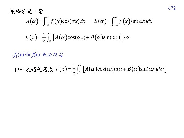
627 11. 2. 4 Conditions for Convergence 其實未必成立 If (1) f 1(x 0) = f(x 0) if f(x) is continuous at x 0
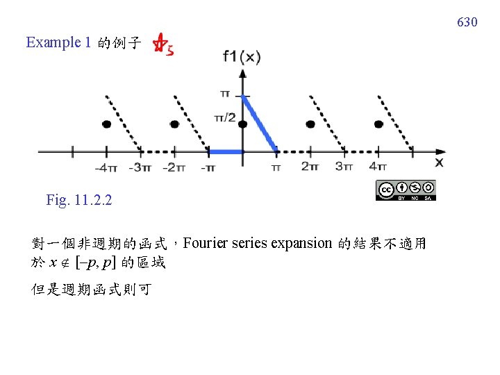
628 (2) Example 1 的例子 Fig. 11 -2 -1 if f(x) is not continuous at x 0
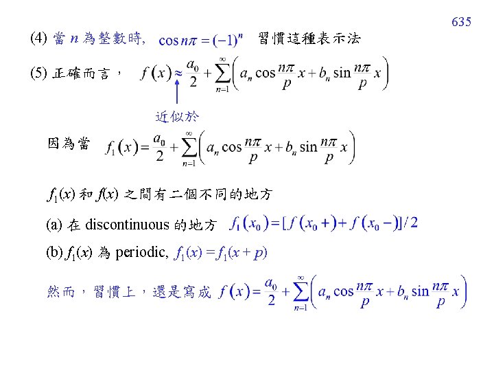
629 11. 2. 5 Period Extension fundamental period: 2 p 在 interval x [ p, p] 以外的地方 (period Extension) f 1(x) 是個週期為 2 p 的 函式 (這是 f 1(x) 和 f(x) 第二個 不同的地方
11. 2. 6 Sequence of Partial Sums N 越大,越能逼近原來的 function 631
632 (a) S 3(x) Fig. 11. 2. 3 (b) S 8(x)
633 (c) S 15(x) Fig. 11. 2. 3 N = 15
637 Section 11. 3 Fourier Cosine and Sine Series 11. 3. 1 綱要 (1) f(x) is even Fourier cosine series (或 cosine series) Fourier Series 比較 page 637 和 page 616 f(x) is odd Fourier sine series (或 sine series)
(2) 重要名詞: Fourier cosine series, cosine series (page 643) Fourier sine series, sine series (page 644) Gibb’s Phenomenon (page 647) 638 (3) Half-range extension: [0, L] (a) cosine series: f(x) = f(−x), interval is changed into [−L, L], set p = L (b) sine series: f(x) = −f(−x), interval is changed into [−L, L ], set p = L (c) Fourier series: (i) interval [−p, p] is replaced by [0, L], (ii) p is replaced by L/2 (4) One of the applications: Solving particular solution (See page 657)
639 11. 3. 2 Even and Odd Functions even function: f(x) = f( x) odd function: f(x) = f( x) Example 1, x 2, x 4, x 6, x 8 …. . are even x, x 3, x 5, x 7, x 9…. . are odd
640 Cosine functions are even cos(t) Sine functions are odd sin(t)
Several properties about even and odd functions (a) The product of two even functions is even 例: x 2 x 4 = x 6 (b) The product of two odd functions is even 例: x x = x 2 (c) The product of an even function and an odd function is odd 例: x x 2 = x 3 (d) The sum (or difference) of two even function is still even (e) The sum (or difference) of two odd function is still odd 641
642 (f) If f(x) is even, then (g) If f(x) is odd, then (Proof): (令 x 1 = −x, dx 1 = −dx) When f(x) = f(−x) When f(x) = − f(−x)
11. 3. 3 Fourier Cosine and Sine Series (1) The Fourier series of an even function on the interval (−p, p) is the cosine series (或稱作 Fourier cosine series) 和之前 Fourier series 不一樣的地方有三個 適用情形: (1) f(x) is even (2) Half range extension (page 649) 643
644 (2) The Fourier series of an odd function on the interval (−p, p) is the sine series (或稱作 Fourier sine series) 和之前 Fourier series 不一樣的地方有三個 (是哪三個) 適用情形: (1) f(x) is odd (2) Half range extension (page 649)
645 Example 1 (text page 438) Expand f(x) = x, 2 < x < 2 in a Fourier series f(x) is odd expand f(x) by a Fourier sine series Fig. 11. 3. 3
646 Example 2 (text page 438) odd function, 使用 sine series Fig. 11. 3. 5
11. 3. 4 Gibbs Phenomenon Example 2 的結果 partial sum 當 N 不為無限大,在 discontinuities 附近會有 “overshooting” 的大小不會隨著 N 而變小 但寬度會越來越窄,越來越靠近 discontinuities 的地方 這種現象,稱作 Gibb’s phenomenon 647
648 (a) S 1(x) (c) S 3(x) Fig. 11. 3. 6 (b) S 2(x) (d) S 15(x)
11. 3. 5 Half Range Extension 649 之前的例子: f(x) is defined in the interval of −p < x < p 若問題改成 Expand f(x), 0 < x < L (f(x) 只有在 0 < x < L 當中有定義) (a) In a cosine series (i) Interval: [−L, L], (ii) 所有公式的 p 由 L 取代, (iii) 結果是 even (b) in a sine series (i) Interval: [−L, L], (ii) 所有公式的 p 由 L 取代 , (iii) 結果是 odd (c) in a Fourier series (i) Interval: [0, L], (ii) 所有公式的 p 由 L/2 取代
650 如 Example 3 (text page 440), f(x) = x 2, 0<x<L (a) in a cosine series 假設 f(x) = f( x) for −L < x < 0, (假設 f(x) 是一個 even function) interval變為 ( L, L) 原本 cosine series 公式 現在只不過將 p 改成 L
651 (b) in a sine series 假設 f(x) = f( x) for −L < x < 0, (假設 f(x) 是一個 odd function) interval 變為 ( L, L) 原本 sine series 公式 現在只不過將 p 改成 L
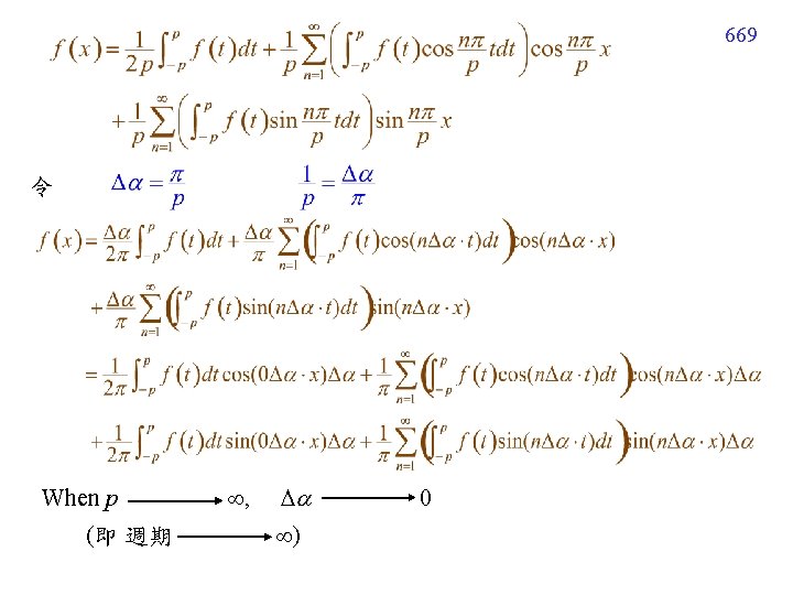
(c) in a Fourier series interval 仍為 (0, L) 原本 Fourier series 公式 現在 (1) 將 interval [−p, p] 換為 [0, L], (2) 將 p 換為 L/2 652
653 Example 3, f(x) = x 2, 0 < x < L 將三個方法的結果畫成圖形 cosine series
654 Fourier series
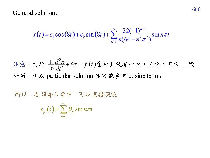
11. 3. 6 Solving Particular Solutions (第四個方法) 方法的限制 (註:以下的步驟不包含解 homogeneous solution 還是需要用 Section 4 -3 的方法來解) (Step 1) 將 f(t) 表示成 Fourier series 或 cosine series (當 f(t) 為 even) 或 sine series (當 f(t) 為 odd) 655
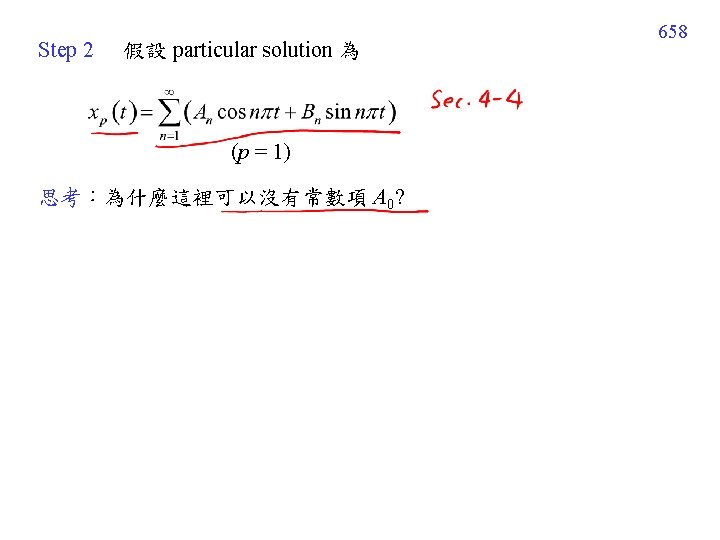
(Step 2) 假設 particular solution 的型態為 (Step 3) 代回原式,比較係數,將 A 0, An, Bn 解出來 若所假設的 particular solution 和 homogeneous solution 有相同的地方,則要乘上 t 656
657 Example 4 (text page 441) (相關物理定理請複習 Section 5. 1) for 1 < t < 1 Step 1 假設 (因為 f(t) 是 odd)
659 Step 3 將 xp(t) 和 Step 1 的結果代入 Therefore, the particular solution is:
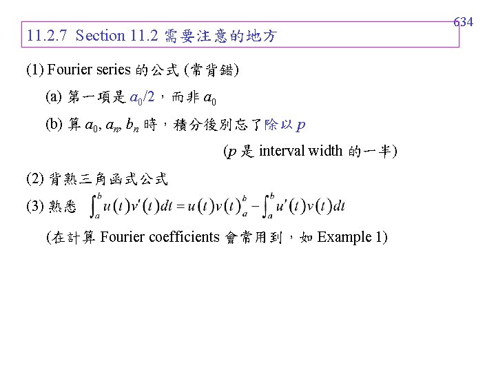
11. 3. 7 Section 11. 3 需要注意的地方 (1) 公式一些地方易記錯 for cosine series and sine series, (2) Fourier series 的 half-range extension 和 cosine series 及 sine series 不同 p is replaced by L/2, [−p, p] is replaced by [0, L] (3) Half range extension 和 solving particular solution 這兩個部分 較複雜,需要特別注意,並且多練習例題 661
662 Exercise for Practice Section 11 -1 3, 5, 6, 8, 13, 14, 17, 19, 20, 21, 22, 23 Section 11 -2 2, 5, 9, 10, 12, 16, 19, 22, 23, 24 Section 11 -3 14, 16, 18, 21, 22, 23, 28, 29, 33, 36, 37, 43, 46, 47 a, 48 a, 49, 52 Review 11 6, 12, 13, 14, 15, 17, 18
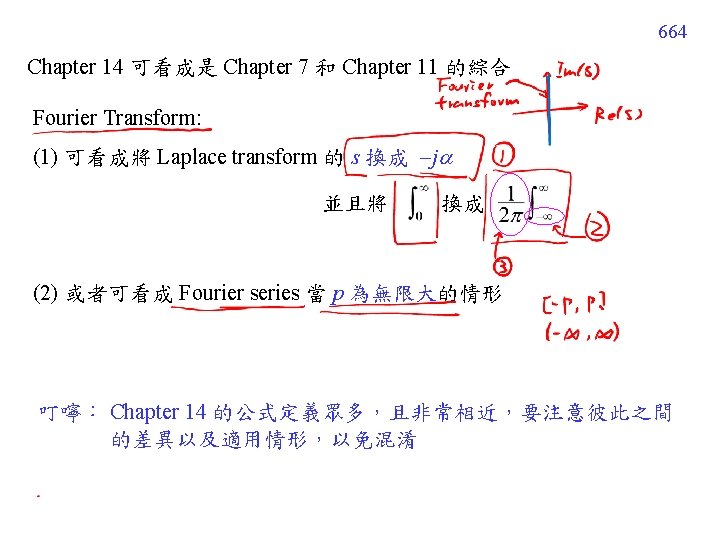
663 Chapter 14 Integral Transform Method Integral transform 可以表示成如下的積分式的 transform kernel Laplace transform is one of the integral transform 本章討論的 integral transform: Fourier transform
Section 14. 3 Fourier Integral 14. 3. 1 綱要 (1) Fourier integral: (和 Fourier series 的定義比較) 665
(2) complex form 或 exponential form of Fourier integral 比較: Fourier integral 原本的定義 666
(3) Fourier cosine integral 或 cosine integral 適用情形: (1) even 或 (2) interval: [0, ) (4) Fourier sine integral 或 sine integral 適用情形: (1) odd 或 (2) interval: [0, ) (5) Others 名詞:absolutely integrable (page 671) partial integral (page 683) 特殊公式: 667
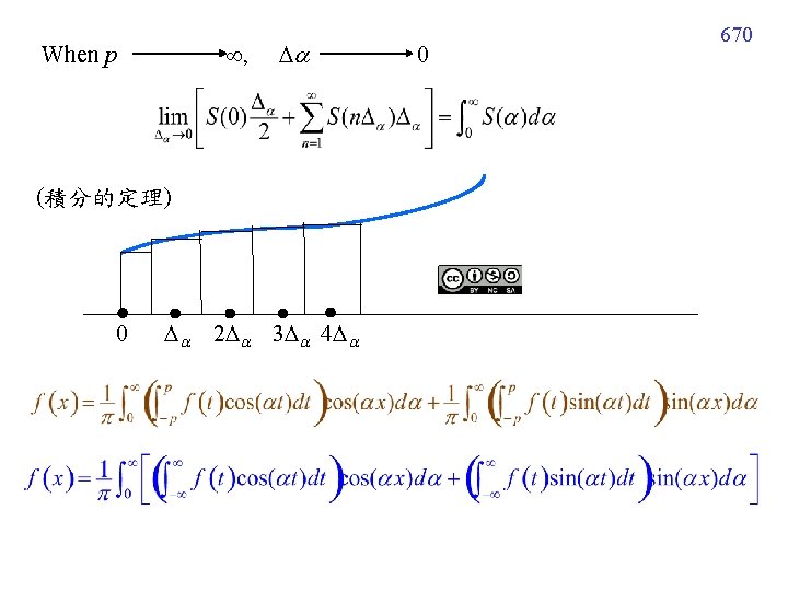
14. 3. 2 From Fourier Series to Fourier Integral 複習:Section 11 -2 的 Fourier series: 668
14. 3. 3 Fourier Integral: Fourier integral 存在的 sufficient condition: converges 若這個條件滿足,f(x) 為 absolutely integrable 671
Theorem 14. 3. 1 Condition for convergence When (1) f(x) 為 piecewise continuous (2) f (x) 為 piecewise continuous (3) f(x) 為 absolutely integrable The Fourier integral of f(x) (即上一頁的 f 1(x)) converges to f(x) at a point of continuity. At the point of discontinuity, f 1(x) converges to 673
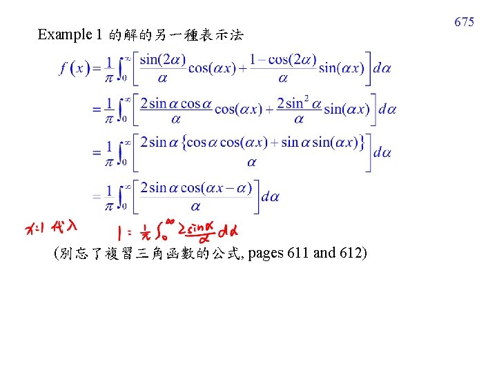
Example 1 (text page 531) Find the Fourier integral representation of f(x) 674
14. 3. 4 Fourier Transform 意外的提供了一些方程式積分的 算法 由 Example 1 When x = 1, since f(x) = 1 676
677 補充: sinc function 的定義: 常用在 sampling theory, filter design, 及通訊上
14. 3. 5 Fourier Cosine and Sine Integrals 678 (A) Fourier cosine integral 或 cosine integral 注意:有三個地方和 Fourier integral 不同 (1) 類比於 cosine series (2) (3) 適用情形: (1) f(x) is even, f(x) = f(−x) (2) 只知道 f(x) 當 x > 0 的時候的值 (類似於Section 11. 3 的 half-range expansion, 而且假設 f(x) = f(−x) )
679 (B) Fourier sine integral 或 sine integral 類比於 sine series 適用情形: (1) f(x) is odd, f(x) = −f(−x) (2) 只知道 f(x) 當 x > 0 的時候的值 (類比於Section 11. 3 的 half-range expansion, 而且假設 f(x) = −f(−x) )
Example 3 (text page 533) Represent (a) by a cosine integral (b) by a sine integral Solution: (a) Suppose that (其實,有一個取巧的快速算法,用 Laplace transform) 680
cosine integral: (b) 681
682 (a) Fig. 14. 3. 4 (b)
683 14. 3. 6 Partial Integral partial integral for Fourier integral partial integral for cosine integral partial integral for sine integral (用 b 取代 )
684 For Example 3 (a) F 5(x) (b) F 20(x) (b = 5) (b = 20) Fig. 14. 3. 5
14. 3. 7 Complex Form complex form or exponential form of Fourier integral remember: 685
686 Proof: 由講義 page 671 Fourier integral 的定義 注意: 對 而言是 even function
687 From (因為 對 而言是 odd function)
688 14. 3. 8 Section 14. 3 需要注意的地方 (1) 公式積分的外面,要乘 (Fourier integral) 或 (Complex form of Fourier integral) 或 (cosine integral, sine integral) (2) 一些積分的計算會常常用到 算法:假設解為 或者用 Laplace transform 的公式, s = 1
Section 14. 4 Fourier Transforms 689 14. 4. 1 綱要 Fourier transform,其實就是 complex form of Fourier integral 公式: 代表 Fourier transform 本節著重於 (1) 定義 (2) 性質 學習方式:多和 Laplace transform 比較 (3) Solving the boundary value problem (pages 703713) 有一點複雜,且常考,要勤於練習
690 (A) 六大定義 (1) Fourier transform (2) inverse Fourier transform (3) Fourier sine transform (4) inverse Fourier sine transform (5) Fourier cosine transform (6) inverse Fourier cosine transform 注意:除了 ej x 變成 cos( x) 以外 還有三個地方和 Fourier transform 不同
691 (B) 微分性質 (7) for Fourier transform (8) (9) for Fourier sine transform 不同 (10) (11) for Fourier cosine transform 不同 (12)
(C) Problems with boundary conditions (多練習) (13) 可考慮用 Fourier transform 的情形 (14) 可考慮用 Fourier sine transform 的情形 when x = 0 (15) 可考慮用 Fourier cosine transform 的情形 另外,要熟悉 page 704 的計算流程 (D) 名詞 transform pair (page 693) heat equation (page 705) 692
693 14. 4. 2 Transform Pair Transform pair 的定義: 若 甲 A 乙 乙 則 A 和 B 形成一個 transform pair 甲和乙 B 甲
694 14. 4. 3 Fourier Transform Fourier transform pair 和之前 complex form of Fourier integral 相比較 只不過把 C( ) 換成 F( ) 為何要取兩個名字? ? ? Fourier transform 存在的條件 (1) (absolutely integrable) (2) f(x) and f (x) 為 piecewise continuous
695 Fourier transform 和 Laplace transform 之間的關係: 把 s 換成 −j Laplace:
14. 4. 4 Fourier Sine Transform and Fourier Cosine Transform Fourier sine transform pair Fourier cosine transform pair Fourier sine / cosine transform 存在的條件 (1) (absolutely integrable) (2) f(x) and f (x) 為 piecewise continuous 696
Fourier sine / cosine transform 的意義: (1)當 f(x) 為 even Fourier transform Fourier cosine transform 等於 0 for Fourier cosine transform 697
698 (2) Inverse Fourier transform inverse Fourier cosine transform If f(x) is even (由前頁) 由於對 Fourier cosine transform 而言 (even function ) 等於 0
Fourier cosine transform 等同於 Fourier transform 當 input f(x) 為 even 的情形。當 f(x) 為 even, Fourier sine transform 等同於 Fourier transform 當 input f(x) 為 odd 的情形。當 f(x) 為 odd, 然而,若 f(x) 只有在 x [0, ) 之間有定義,也可以用 Fourier cosine / sine transform (類似於Section 11. 3 的 half-range expansion) 699
14. 4. 5 微分性質 (1) Fourier transform 的微分性質做了一些假設: f(x) = 0 when x and x 以此類推 比較:對 Laplace transform 對 Fourier transform s −j , without initial conditions 700
(2) Fourier sine transform 的微分性質 (3) Fourier cosine transform 的微分性質 注意: (1) Fourier sine, cosine transforms 互換 (2) 正負號不同 (3) Fourier cosine transform 要考慮 initial condition 701
702
14. 4. 6 Solving the Boundary Value Problem (BVP) 703 ※ 概念複雜,要特別加強練習 (Condition 1) interval 為 < v < 時: 用 Fourier transform (Condition 2) interval 為 0 < v < , 有 “u(v, …. . ) = 0 or a constant when v = 0” 的 boundary condition 時 : 用 Fourier sine transform (Condition 3) interval 為 0 < v < , 有“ 時: or a constant when v = 0” 的 boundary condition 用 Fourier cosine transform
使 用 Fourier transform, Fourier cosine transform, Fourier sine transform 來解 partial differential equation (PDE) 的 BVP 或IVP 的解法流程 (Step 1) 以 page 703 的規則,來決定要針對 哪一個 independent variable ,做什麼 transform (Fourier, Fourier cosine, 或Fourier sine transform) (Step 2) 對 PDE 做 Step 1 所決定的 transform, 則原本的 PDE 變成 針對另外一個 independent variable 的 ordinary differential equation (ODE) (Step 3) 將 Step 2 所得出的 ODE 的解算出來 (Step 4) Step 3 所得出來的解會有一些 constants,可以對 initial conditions (或 boundary conditions) 做 transform 將 constants 解出 (※ 和 Step 1 所做的 transform 一樣,只是 transform 的對象變成 是 initial 或 boundary conditions,見 pages 705, 708 的例子) (Step 5) 最後,別忘了做 inverse transform (畫龍點睛) 704
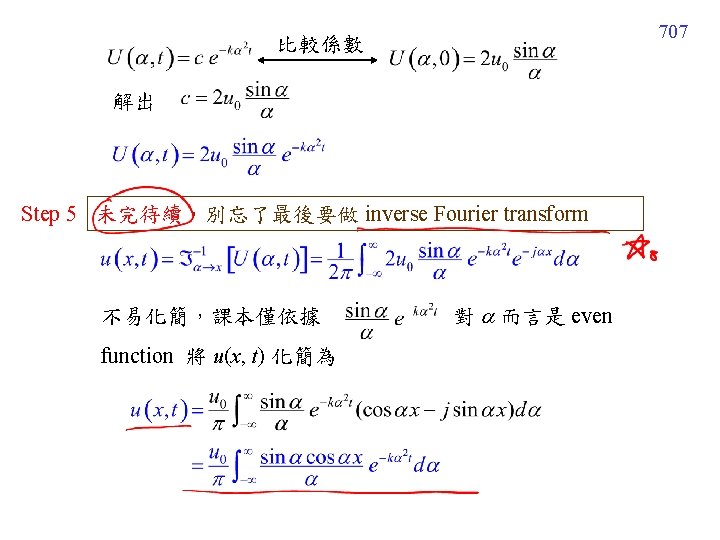
705 Example 1 (text page 538) heat equation: subject to where Step 1 決定針對 x 做 Fourier transform Step 2 原本對 x, t 兩個變數做偏微分 經過 Fourier transform 之後, 只剩下對 t 做偏微分
706 對於 t 而言,是 1 st order ODE 這邊的 c 值,對 t 而言是 constant , Step 3 但是可能會 dependent on (特別注意) Step 4 根據 u(x, 0) = f(x) 將 c 解出 和 Step 1 一樣,也是針對 x 做 Fourier transform 只是對象改成 initial condition 因為
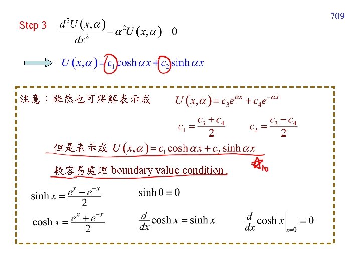
Example 3 Laplace’s equation (text page 540) Step 1 決定針對 y 做 Fourier cosine transform Step 2 from 對於 x 的 2 nd order ODE 708
710 Step 4 由 來解 c 1, c 2 和 Step 1 一樣,也是針對 y 做 Fourier cosine transform 只是對象改成 boundary conditions (1 ) (2 ) 分別代入 (1 ) (2 ) (可以用Laplace transform 的「取巧法」 )
711 Step 5 inverse cosine transform (算到這裡即可,難以繼續化簡)
14. 4. 7 Section 14. 4 需要注意的地方 712 (1) 微分公式當中,Fourier cosine transform 和 Fourier sine transform 會 有互換的情形。(See pages 701, 702) (2) 公式會有很多小地方會背錯 (特別注意綱要的公式中紅色的地方) (3) 在解 boundary value problem 時,要了解 何時用 Fourier transform, 何時用Fourier cosine transform, 何時用 Fourier sine transform (see page 703) (4) 解 boundary value problem 流程雖複雜,但只要記住, 方法的精神,在於: 運用 transform, 將原本針對兩個以上 independent variables 做微分的 PDE, 變成只有針對一個 independent variable 做微分的 ODE
713 (5) 在解 partial differential equation 時,往往只針對一個 independent variable 做 Fourier transform, 另一個 independent variable 不受影響, 如 Examples 1 and 2, pages 705 and 708 的例子 計算過程中,自己要清楚是對哪一個 independent variable 做Fourier transform ※ 本人習慣用下標做記號 (建議同學們使用) (6) Step 4 和 Step 1 必需是針對同一個 independent variable 來做 同一種 transform,只是處理的對象改成了 initial (or boundary) conditions (see pages 706, 710) (7) 注意 page 709, 有時我們會用 來取代 ,以方便計算
716 Exercise for Practice Section 14 -3 3, 4, 7, 12, 15, 16, 17, 19, 20 Section 14 -4 1, 2, 3, 9, 12, 15, 16, 18, 19, 20, 21, 27 Review 14 2, 7, 8, 11, 15, 16