Discrete Fourier Transform The Discrete Fourier Transform is

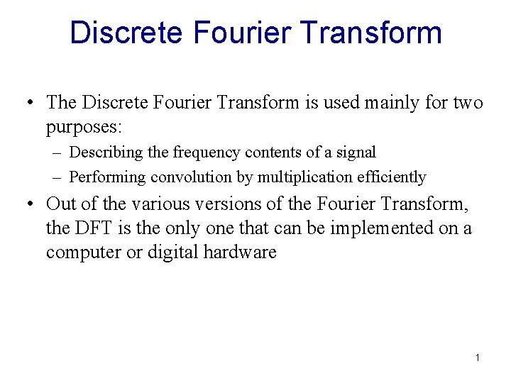
Discrete Fourier Transform • The Discrete Fourier Transform is used mainly for two purposes: – Describing the frequency contents of a signal – Performing convolution by multiplication efficiently • Out of the various versions of the Fourier Transform, the DFT is the only one that can be implemented on a computer or digital hardware 1

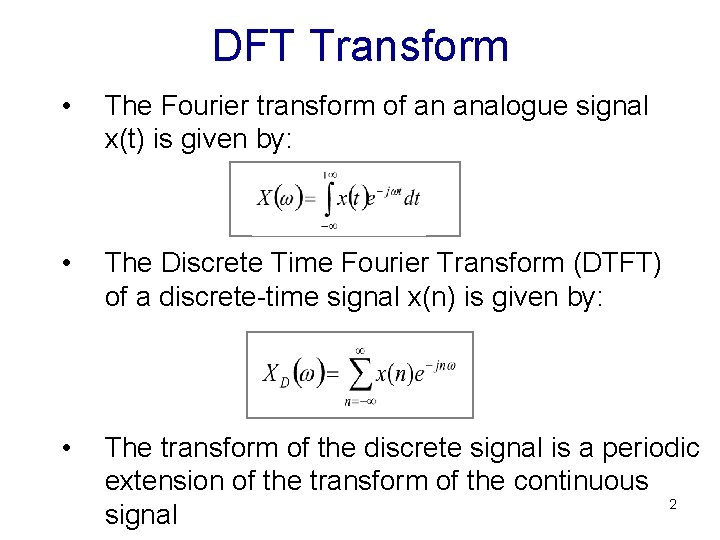
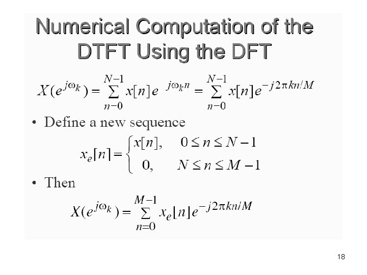
DFT Transform • The Fourier transform of an analogue signal x(t) is given by: • The Discrete Time Fourier Transform (DTFT) of a discrete-time signal x(n) is given by: • The transform of the discrete signal is a periodic extension of the transform of the continuous 2 signal

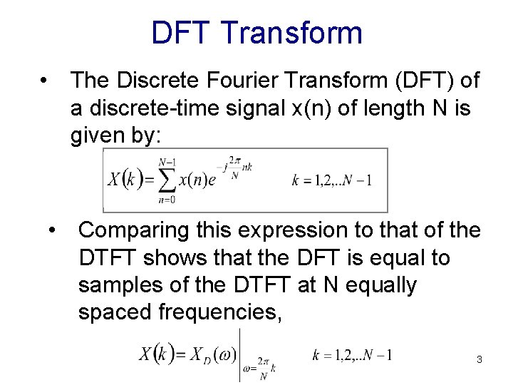
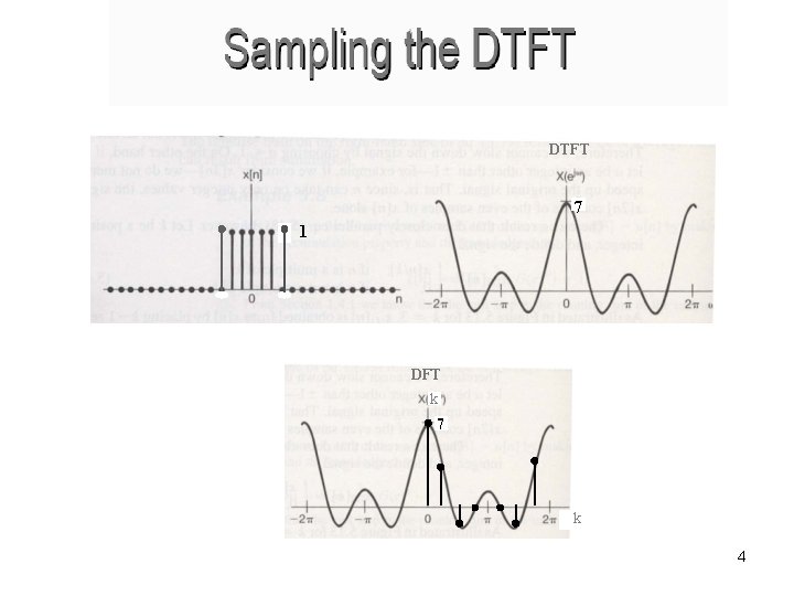
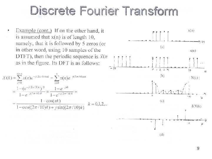
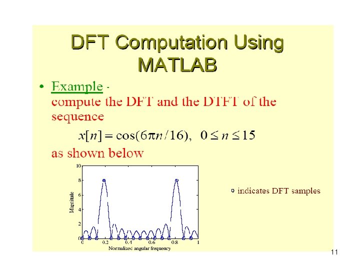
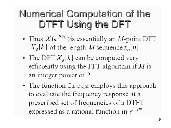
DFT Transform • The Discrete Fourier Transform (DFT) of a discrete-time signal x(n) of length N is given by: • Comparing this expression to that of the DTFT shows that the DFT is equal to samples of the DTFT at N equally spaced frequencies, 3

DTFT 7 1 DFT k 7 k 4

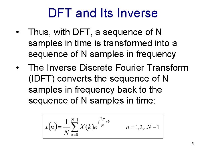
DFT and Its Inverse • Thus, with DFT, a sequence of N samples in time is transformed into a sequence of N samples in frequency • The Inverse Discrete Fourier Transform (IDFT) converts the sequence of N samples in frequency back to the sequence of N samples in time: 5

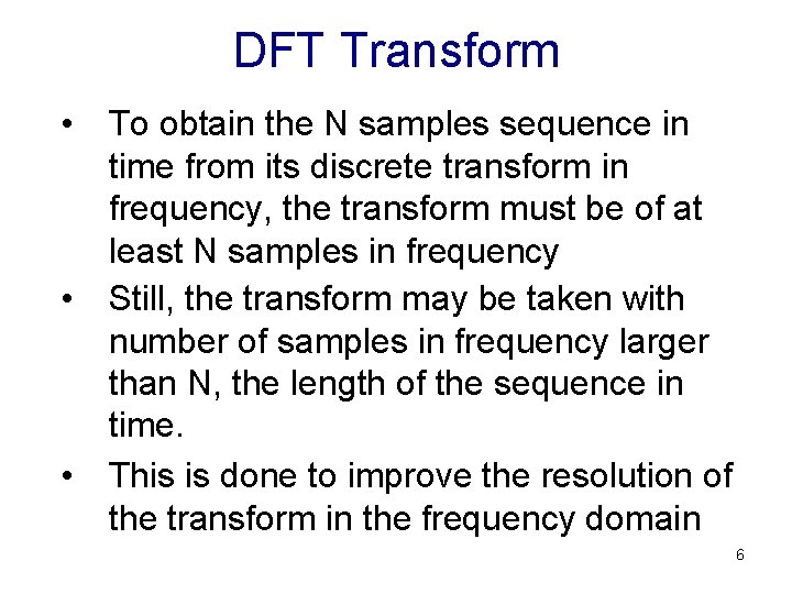
DFT Transform • To obtain the N samples sequence in time from its discrete transform in frequency, the transform must be of at least N samples in frequency • Still, the transform may be taken with number of samples in frequency larger than N, the length of the sequence in time. • This is done to improve the resolution of the transform in the frequency domain 6

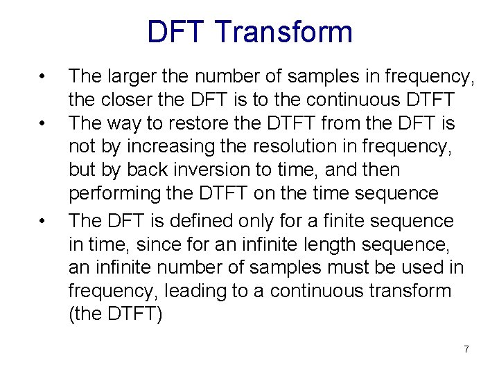
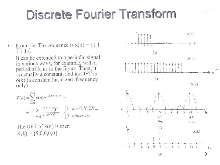
DFT Transform • • • The larger the number of samples in frequency, the closer the DFT is to the continuous DTFT The way to restore the DTFT from the DFT is not by increasing the resolution in frequency, but by back inversion to time, and then performing the DTFT on the time sequence The DFT is defined only for a finite sequence in time, since for an infinite length sequence, an infinite number of samples must be used in frequency, leading to a continuous transform (the DTFT) 7

x(n) (a) x(n) (b) X(k) (c) X(k) (d) 8

9

10

11

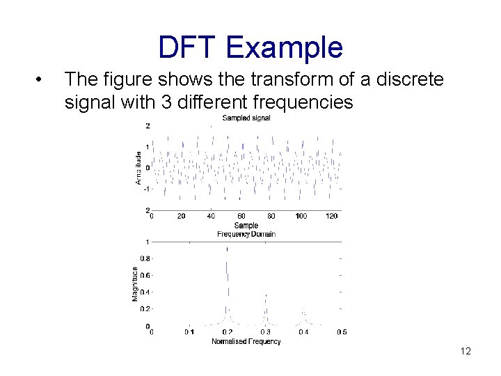
DFT Example • The figure shows the transform of a discrete signal with 3 different frequencies 12

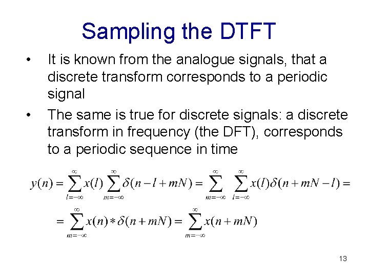
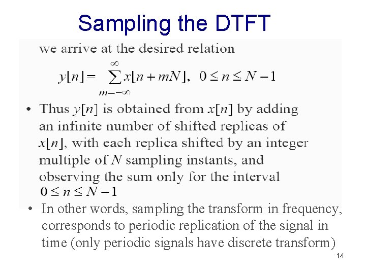
Sampling the DTFT • • It is known from the analogue signals, that a discrete transform corresponds to a periodic signal The same is true for discrete signals: a discrete transform in frequency (the DFT), corresponds to a periodic sequence in time 13

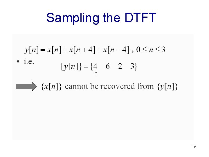
Sampling the DTFT • In other words, sampling the transform in frequency, corresponds to periodic replication of the signal in time (only periodic signals have discrete transform) 14

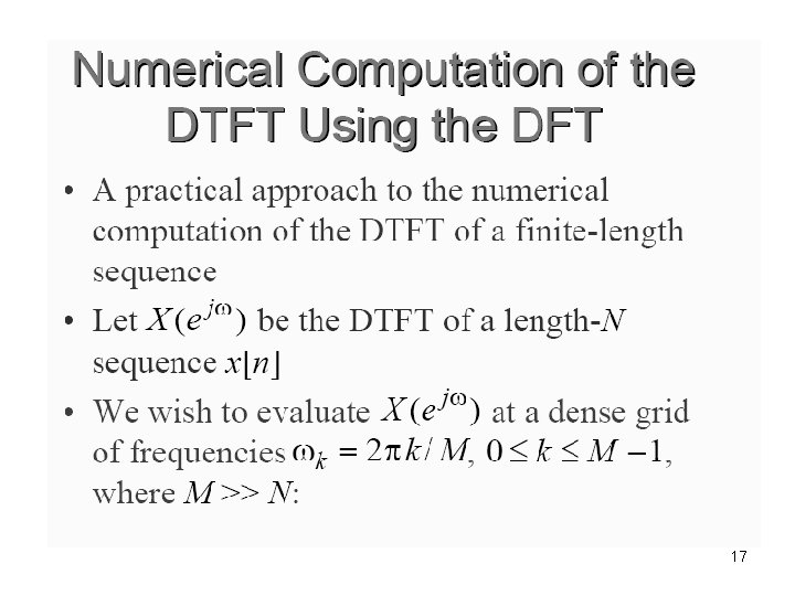
Sampling the DTFT Here, M is the length of x[n], and N is the number samples taken in the frequency domain 15

Sampling the DTFT 16

17

18

19

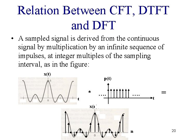
Relation Between CFT, DTFT and DFT • A sampled signal is derived from the continuous signal by multiplication by an infinite sequence of impulses, at integer multiples of the sampling interval, as in the figure: x(t) p(t) t * …. t = x(n) n 20

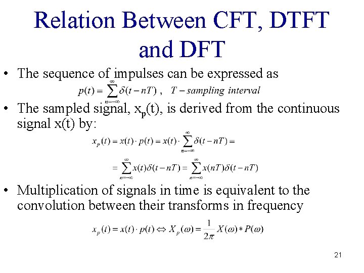
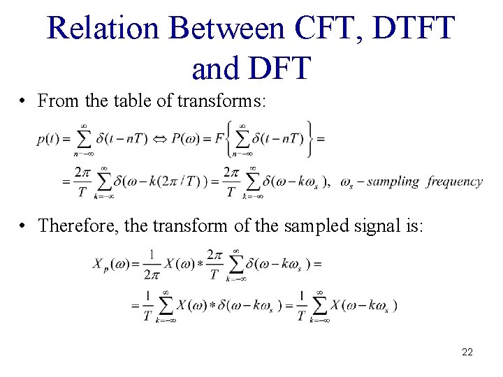
Relation Between CFT, DTFT and DFT • The sequence of impulses can be expressed as • The sampled signal, xp(t), is derived from the continuous signal x(t) by: • Multiplication of signals in time is equivalent to the convolution between their transforms in frequency 21

Relation Between CFT, DTFT and DFT • From the table of transforms: • Therefore, the transform of the sampled signal is: 22

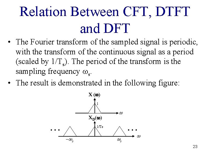
Relation Between CFT, DTFT and DFT • The Fourier transform of the sampled signal is periodic, with the transform of the continuous signal as a period (scaled by 1/Ts). The period of the transform is the sampling frequency ws. • The result is demonstrated in the following figure: X (w) 1 XD(w) … w … 1/Ts -ws ws w 23

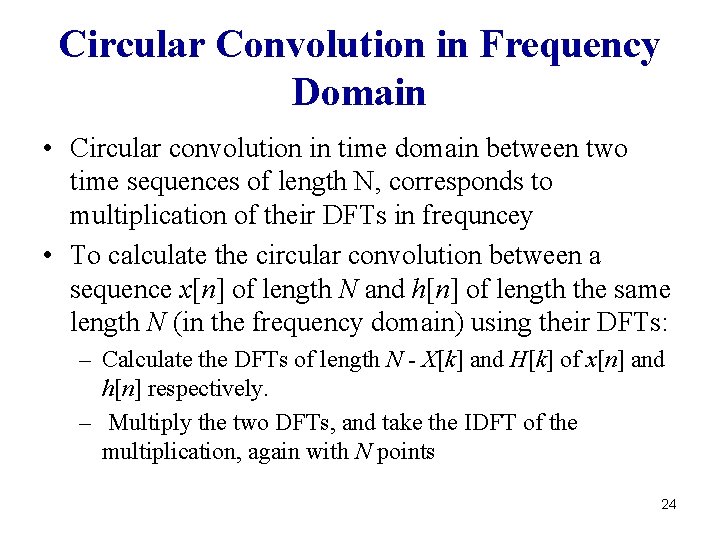
Circular Convolution in Frequency Domain • Circular convolution in time domain between two time sequences of length N, corresponds to multiplication of their DFTs in frequncey • To calculate the circular convolution between a sequence x[n] of length N and h[n] of length the same length N (in the frequency domain) using their DFTs: – Calculate the DFTs of length N - X[k] and H[k] of x[n] and h[n] respectively. – Multiply the two DFTs, and take the IDFT of the multiplication, again with N points 24

25

26

27

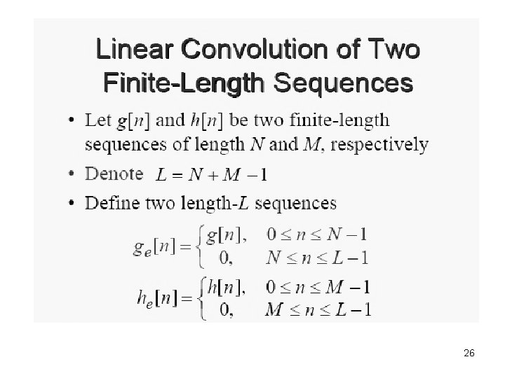
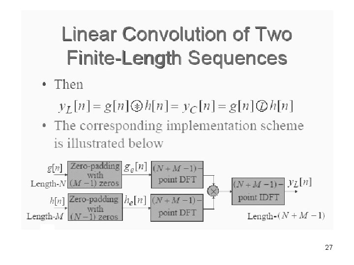
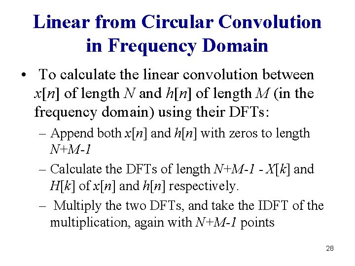
Linear from Circular Convolution in Frequency Domain • To calculate the linear convolution between x[n] of length N and h[n] of length M (in the frequency domain) using their DFTs: – Append both x[n] and h[n] with zeros to length N+M-1 – Calculate the DFTs of length N+M-1 - X[k] and H[k] of x[n] and h[n] respectively. – Multiply the two DFTs, and take the IDFT of the multiplication, again with N+M-1 points 28

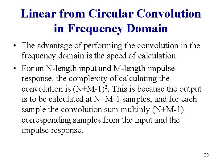
Linear from Circular Convolution in Frequency Domain • The advantage of performing the convolution in the frequency domain is the speed of calculation • For an N-length input and M-length impulse response, the complexity of calculating the convolution is (N+M-1)2. This is because the output is to be calculated at N+M-1 samples, and for each sample the convolution sum multiply (N+M-1) corresponding samples from the input and the impulse response. 29

Linear from Circular Convolution in Frequency Domain • Similar complexity is obtained when performing the convolution in the frequency domain using DFT. The DFT is calculated at (N+M-1) points in frequency, and at each point, the calculation is over (N+M-1) samples (both of input and impulse response) • However, there is a fast implementation of DFT, named FFT (Fast Fourier Transform), which reduces the computational complexity of the DFT to (N+M-1)log(N+M-1) 30

Real-Time DFT Computation • Operations such as DFT or FFT require that a frame of data be present at the time of processing • Unlike filtering , where operations are done on every incoming sample, in frame processing N samples are captured first, and then operations are performed on N samples. • To perform frame processing, a proper method of gathering data and of processing and sending data out is required 31

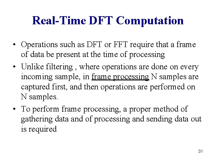
Real-Time DFT Computation • The processing of a frame of data is not usually completed within the sampling time interval. • Rather, it is spread over the duration of a frame, before and while the next frame of data is gathered. • Hence, incoming samples must be stored into a separate buffer, other than the one being processed • Also, another buffer is needed to send out a previously processed frame of data 32

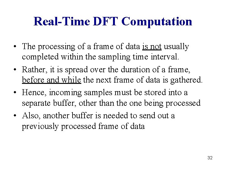
Real-Time DFT Computation • This can be achieved by triple buffering involving three buffers: input, intermediate and output. • The buffers rotate every time the input buffer is full • Then, the new frame of N samples is passed to the intermediate buffer for processing, and a previously processed frame is passed to the output buffer for transmission. 33

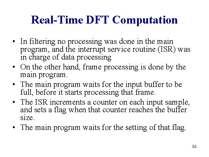
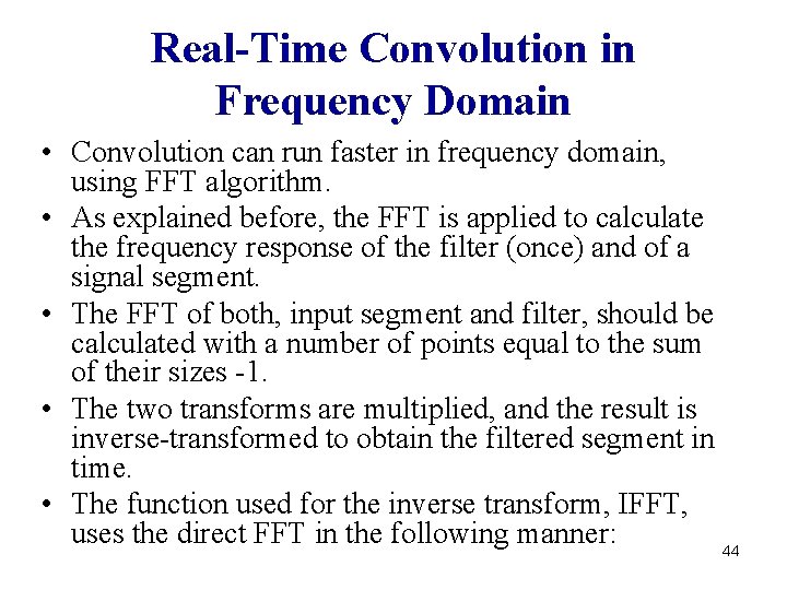
Real-Time DFT Computation • In filtering no processing was done in the main program, and the interrupt service routine (ISR) was in charge of data processing • On the other hand, frame processing is done by the main program. • The main program waits for the input buffer to be full, before it starts processing that frame. • The ISR increments a counter on each input sample, and sets a flag when that counter reaches the buffer size. • The main program waits for the setting of that flag. 34

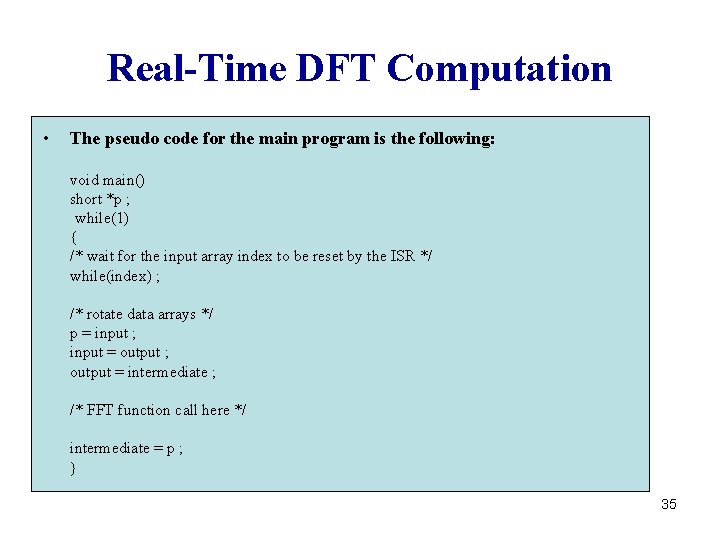
Real-Time DFT Computation • The pseudo code for the main program is the following: void main() short *p ; while(1) { /* wait for the input array index to be reset by the ISR */ while(index) ; /* rotate data arrays */ p = input ; input = output ; output = intermediate ; /* FFT function call here */ intermediate = p ; } 35

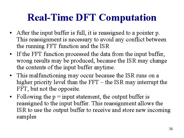
Real-Time DFT Computation • After the input buffer is full, it is reassigned to a pointer p. This reassignment is necessary to avoid any conflict between the running FFT function and the ISR • If the FFT function processed the data from the input buffer, wrong results may be produced, because the ISR may change the contents of the input buffer anytime. • This malfunctioning may occur because the ISR runs on a higher priority level than the FFT – the ISR may interrupt the FFT, but not the opposite. • Following the p = input statement, the output buffer is reassigned to the input buffer. This reassignment allows the ISR to use the output buffer to receive and store new incoming samples 36

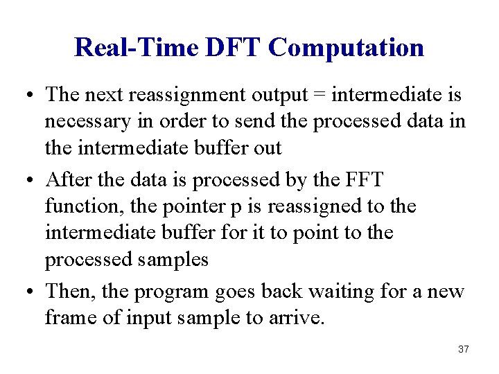
Real-Time DFT Computation • The next reassignment output = intermediate is necessary in order to send the processed data in the intermediate buffer out • After the data is processed by the FFT function, the pointer p is reassigned to the intermediate buffer for it to point to the processed samples • Then, the program goes back waiting for a new frame of input sample to arrive. 37

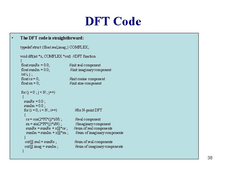
DFT Code • The DFT code is straightforward: typedef struct {float real, imag; } COMPLEX; void dft(int *x, COMPLEX *out) //DFT function { float sum. Re = 0. 0; //init real component float sum. Im = 0. 0; //init imaginary component i, j ; float cs = 0; //init cosine component float sn = 0; //init sine component for (j = 0 ; j < N ; j++) { sum. Re = 0. 0 ; sum. Im = 0. 0 ; for (i = 0; i < N ; i++) { cs = cos(2*PI*(j)*i/N) ; sn = sin(2*PI*(j)*i/N) ; sum. Re = sum. Re + x[i]*cs ; sum. Im = sum. Im + x[i]*sn ; } out[j]. real = sum. Re ; out[j]. imag = sum. Im ; } //for N-point DFT //real component //imaginary component //sum of real components //sum of imaginary components 38

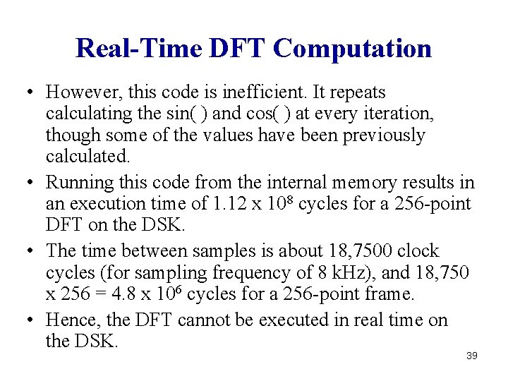
Real-Time DFT Computation • However, this code is inefficient. It repeats calculating the sin( ) and cos( ) at every iteration, though some of the values have been previously calculated. • Running this code from the internal memory results in an execution time of 1. 12 x 108 cycles for a 256 -point DFT on the DSK. • The time between samples is about 18, 7500 clock cycles (for sampling frequency of 8 k. Hz), and 18, 750 x 256 = 4. 8 x 106 cycles for a 256 -point frame. • Hence, the DFT cannot be executed in real time on the DSK. 39

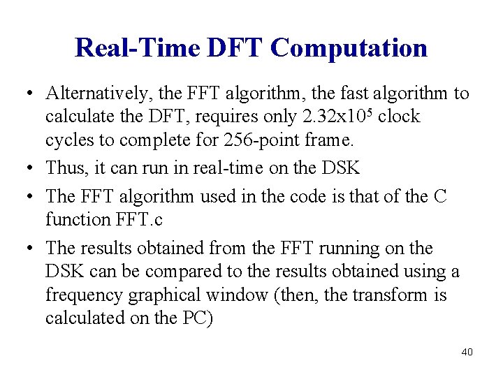
Real-Time DFT Computation • Alternatively, the FFT algorithm, the fast algorithm to calculate the DFT, requires only 2. 32 x 105 clock cycles to complete for 256 -point frame. • Thus, it can run in real-time on the DSK • The FFT algorithm used in the code is that of the C function FFT. c • The results obtained from the FFT running on the DSK can be compared to the results obtained using a frequency graphical window (then, the transform is calculated on the PC) 40

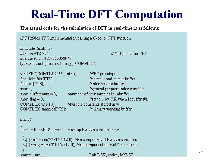
Real-Time DFT Computation The actual code for the calculation of DFT in real-time is as follows: //FFT 256 c. c FFT implementation calling a C-coded FFT function #include <math. h> #define PTS 256 #define PI 3. 14159265358979 typedef struct {float real, imag; } COMPLEX; // # of points for FFT void FFT(COMPLEX *Y, int n); //FFT prototype float iobuffer[PTS]; //as input and output buffer float x 1[PTS]; //intermediate buffer short i; //general purpose index variable short buffercount = 0; //number of new samples in iobuffer short flag = 0; //set to 1 by ISR when iobuffer full COMPLEX w[PTS]; //twiddle constants stored in w COMPLEX samples[PTS]; //primary working buffer main() { for (i = 0 ; i<PTS ; i++) // set up twiddle constants in w { w[i]. real = cos(2*PI*i/512. 0); //Re component of twiddle constants w[i]. imag =-sin(2*PI*i/512. 0); //Im component of twiddle constants } comm_intr(); //init DSK, codec, Mc. BSP 41

Real-Time DFT Computation The code continued : while(1) //infinite loop { while (flag == 0) ; //wait until iobuffer is full flag = 0; //reset flag for (i = 0 ; i < PTS ; i++) //swap buffers { samples[i]. real=iobuffer[i]; //buffer with new data iobuffer[i] = x 1[i]; //processed frame to iobuffer } for (i = 0 ; i < PTS ; i++) samples[i]. imag = 0. 0 ; //imag components = 0 FFT(samples, PTS); //call function FFT. c for (i = 0 ; i < PTS ; i++) //compute magnitude { x 1[i] = sqrt(samples[i]. real*samples[i]. real + samples[i]. imag*samples[i]. imag)/32; } } //end of infinite loop } //end of main 42

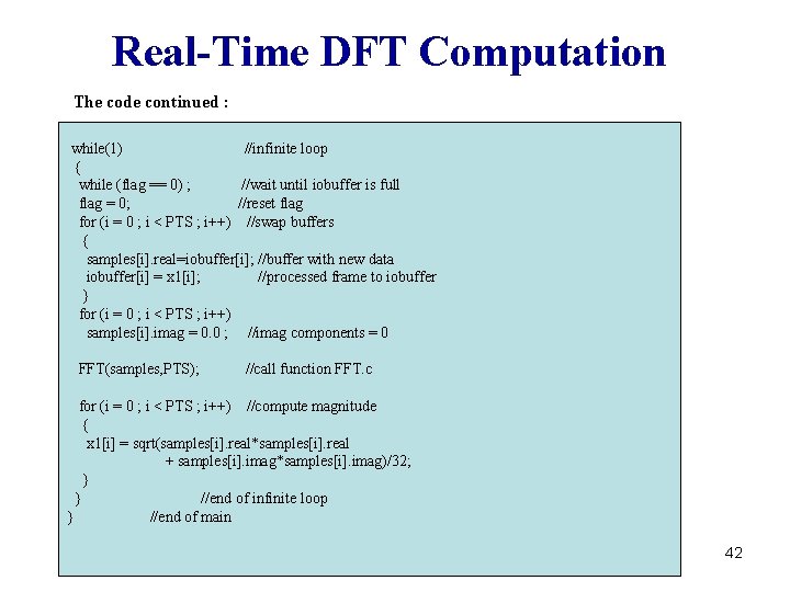
Real-Time DFT Computation The sampling ISR : interrupt void c_int 11() //ISR { output_sample((int)(iobuffer[buffercount])); //out from iobuffer[buffercount++]=(float)(input_sample()); //input to iobuffer if (buffercount >= PTS) //if iobuffer full { buffercount = 0; //reinit buffercount flag = 1; //set flag } } 43

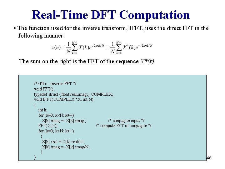
Real-Time Convolution in Frequency Domain • Convolution can run faster in frequency domain, using FFT algorithm. • As explained before, the FFT is applied to calculate the frequency response of the filter (once) and of a signal segment. • The FFT of both, input segment and filter, should be calculated with a number of points equal to the sum of their sizes -1. • The two transforms are multiplied, and the result is inverse-transformed to obtain the filtered segment in time. • The function used for the inverse transform, IFFT, uses the direct FFT in the following manner: 44

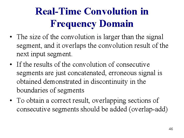
Real-Time DFT Computation • The function used for the inverse transform, IFFT, uses the direct FFT in the following manner: The sum on the right is the FFT of the sequence X*(k) /* ifft. c - inverse FFT */ void FFT(); typedef struct {float real, imag; } COMPLEX; void IFFT(COMPLEX *X, int N) { int k; for (k=0; k<N; k++) X[k]. imag = -X[k]. imag ; /* conjugate input */ FFT(X, N); /* compute FFT of conjugate */ for (k=0; k<N; k++) { X[k]. real = X[k]. real/N ; X[k]. imag = -X[k]. imag/N ; } } 45

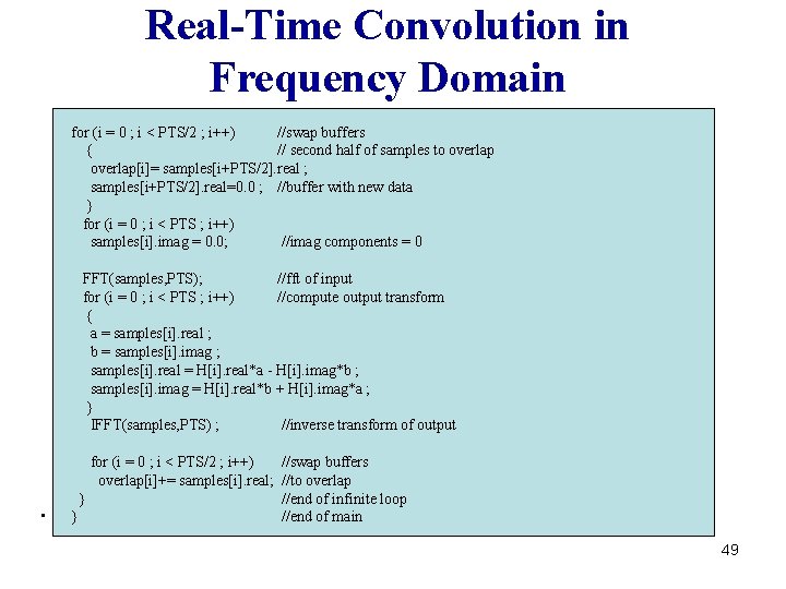
Real-Time Convolution in Frequency Domain • The size of the convolution is larger than the signal segment, and it overlaps the convolution result of the next input segment. • If the results of the convolution of consecutive segments are just concatenated, erroneous signal is obtained demonstrated in discontinuity in the boundaries of segments • To obtain a correct result, overlapping sections of consecutive segments should be added (overlap-add) 46

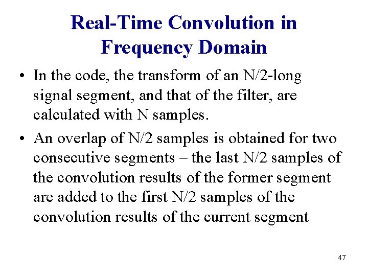
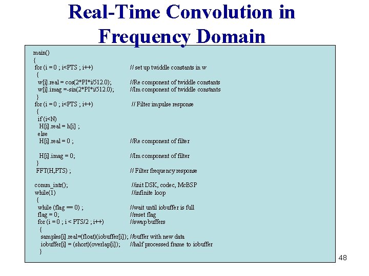
Real-Time Convolution in Frequency Domain • In the code, the transform of an N/2 -long signal segment, and that of the filter, are calculated with N samples. • An overlap of N/2 samples is obtained for two consecutive segments – the last N/2 samples of the convolution results of the former segment are added to the first N/2 samples of the convolution results of the current segment 47

Real-Time Convolution in Frequency Domain • • • • • • • main() { for (i = 0 ; i<PTS ; i++) { w[i]. real = cos(2*PI*i/512. 0); w[i]. imag =-sin(2*PI*i/512. 0); } for (i = 0 ; i<PTS ; i++) { if (i<N) H[i]. real = h[i] ; else H[i]. real = 0 ; // set up twiddle constants in w //Re component of twiddle constants //Im component of twiddle constants // Filter impulse response //Re component of filter H[i]. imag = 0; } FFT(H, PTS) ; //Im component of filter comm_intr(); while(1) { while (flag == 0) ; flag = 0; for (i = 0 ; i < PTS/2 ; i++) { samples[i]. real=(float)(iobuffer[i]); iobuffer[i] = (short)(overlap[i]); } //init DSK, codec, Mc. BSP //infinite loop // Filter frequency response //wait until iobuffer is full //reset flag //swap buffers //buffer with new data //half processed frame to iobuffer 48

Real-Time Convolution in Frequency Domain • • • • • • for (i = 0 ; i < PTS/2 ; i++) //swap buffers { // second half of samples to overlap[i]= samples[i+PTS/2]. real ; samples[i+PTS/2]. real=0. 0 ; //buffer with new data } for (i = 0 ; i < PTS ; i++) samples[i]. imag = 0. 0; //imag components = 0 FFT(samples, PTS); //fft of input for (i = 0 ; i < PTS ; i++) //compute output transform { a = samples[i]. real ; b = samples[i]. imag ; samples[i]. real = H[i]. real*a - H[i]. imag*b ; samples[i]. imag = H[i]. real*b + H[i]. imag*a ; } IFFT(samples, PTS) ; //inverse transform of output for (i = 0 ; i < PTS/2 ; i++) //swap buffers overlap[i]+= samples[i]. real; //to overlap } //end of infinite loop } //end of main 49