Image Transforms WenNung Lie 2 D orthogonal and

Image Transforms Wen-Nung Lie

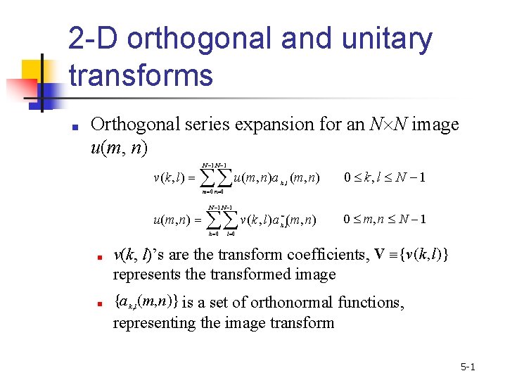
2 -D orthogonal and unitary transforms ■ Orthogonal series expansion for an N N image u(m, n) v(k, l) N 1 u(m, n)a (m, n) 0 k, l N 1 v(k, l)a (m, n) 0 m, n N 1 k , l m 0 n 0 u(m, n) N 1 * k , l k 0 ■ ■ l 0 v(k, l)’s are the transform coefficients, V {v(k, l)} represents the transformed image {a k , l (m, n)} is a set of orthonormal functions, representing the image transform 5 -1

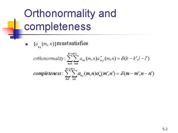
Orthonormality and completeness ■ {a k , l (m, n)}must satisfies N 1 orthonormality : a m 0 k 0 (m, n)a k* , l (m, n) (k k , l l ) n 0 N 1 completeness : k , l a k , l (m, n)a k*, l(m , n ) (m m , n n ) l 0 5 -2

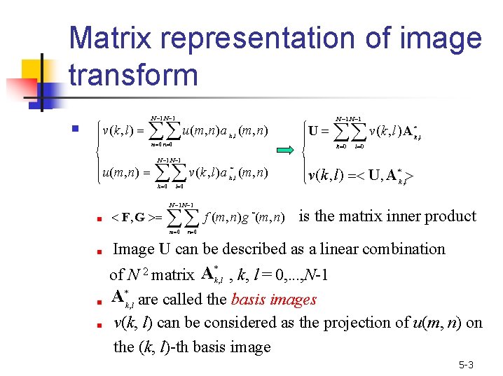
Matrix representation of image transform ■ v(k, l) N 1 u(m, n)a k , l (m, n) m 0 n 0 u(m, n) ■ ■ k 0 F, G v(k, l)a k*, l (m, n) l 0 N 1 f (m, n)g (m, n) * m 0 ■ v(k, l)A * k , l l 0 N 1 k 0 ■ U N 1 v(k, l) U, A *k , l is the matrix inner product n 0 Image U can be described as a linear combination * 2 A of N matrix k , l , k, l = 0, . . . , N-1 A *k , l are called the basis images v(k, l) can be considered as the projection of u(m, n) on the (k, l)-th basis image 5 -3

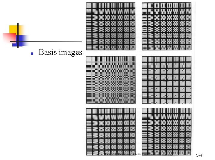
■ Basis images 5 -4

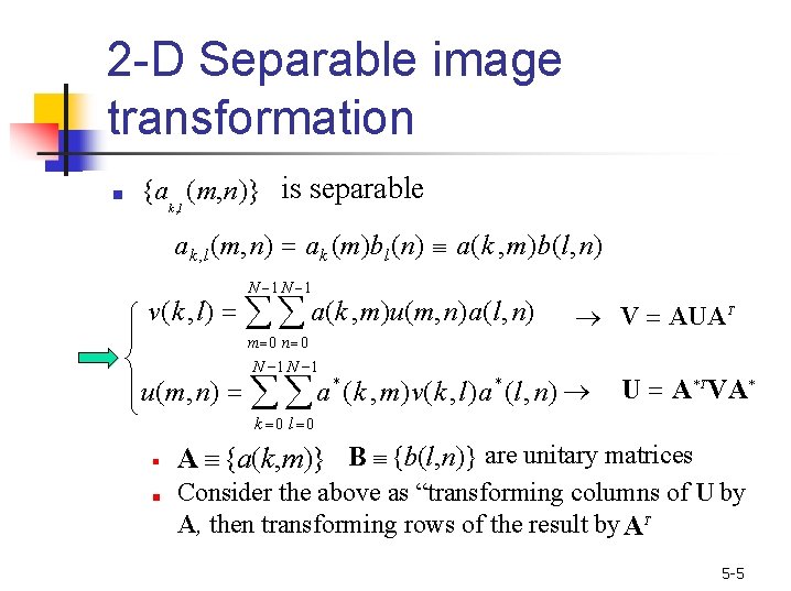
2 -D Separable image transformation ■ {ak , l (m, n)} is separable ak , l (m, n) ak (m)bl (n) a(k , m)b(l, n) N 1 v(k , l) a(k , m)u(m, n)a(l, n) m 0 n 0 N 1 V AUAT u(m, n) a * (k , m)v(k , l)a * (l, n) U A *TVA * k 0 l 0 ■ ■ A {a(k, m)} B {b(l, n)} are unitary matrices Consider the above as “transforming columns of U by A, then transforming rows of the result by A T 5 -5

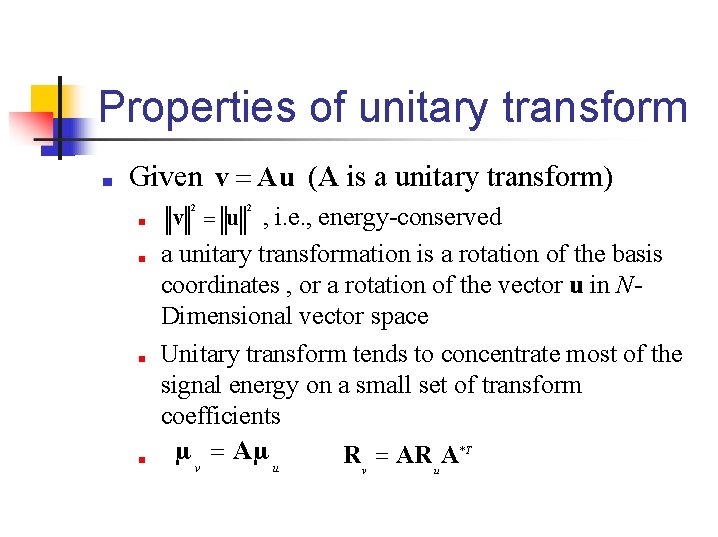
Properties of unitary transform ■ Given v Au (A is a unitary transform) 2 ■ ■ v u 2 , i. e. , energy-conserved a unitary transformation is a rotation of the basis coordinates , or a rotation of the vector u in NDimensional vector space Unitary transform tends to concentrate most of the signal energy on a small set of transform coefficients µ v Aµ u R v AR u A*T

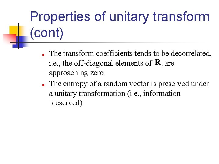
Properties of unitary transform (cont) ■ ■ The transform coefficients tends to be decorrelated, i. e. , the off-diagonal elements of R v are approaching zero The entropy of a random vector is preserved under a unitary transformation (i. e. , information preserved)

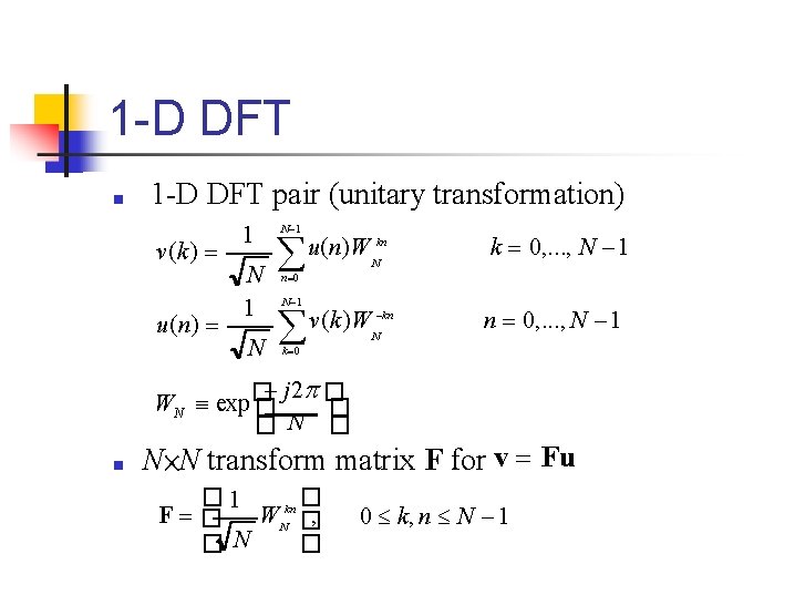
1 -D DFT ■ 1 -D DFT pair (unitary transformation) v(k ) 1 N 1 N u(n)W Nkn k 0, . . . , N 1 1 v(k )WN kn n 0, . . . , N 1 n 0 u(n) N 1 N k 0 j 2 � WN exp� � � �N � ■ N×N transform matrix F for v Fu � 1 � F � WNkn � , � �N 0 k, n N 1

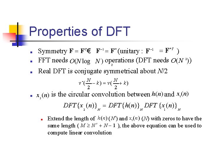
Properties of DFT ■ ■ Symmetry F F T € F 1 F * (unitary : F 1 F *T ) FFT needs O(N log N ) operations (DFT needs O(N 2)) Real DFT is conjugate symmetrical about N/2 2 ■ v*( ■ N N k ) v( k ) 2 2 x 2 (n) is the circular convolution between h(n) and x 1(n) DFT {x 2 (n)} N DFT {h(n)} N DFT {x 1 (n)} N ■ Extend the length of h(n) ( N ) and x (n) (N) with zeros to have the same length ( M N N 1 ), the above equation can be used to compute linear convolution 1

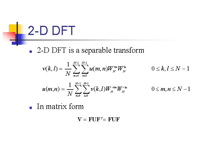
2 -D DFT ■ 2 -D DFT is a separable transform 1 v(k, l) N 1 u(m, n) N ■ N 1 m 0 N 1 u(m, n)W Nkm. W Nln n 0 N 1 v(k, l)W k 0 0 k, l N 1 km N W N ln l 0 In matrix form V FUF T FUF 0 m, n N 1

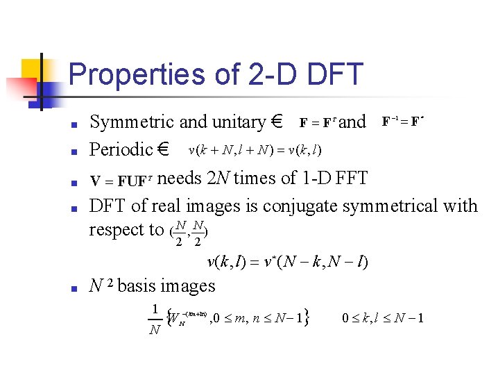
Properties of 2 -D DFT ■ ■ Symmetric and unitary € F F and F F Periodic € v(k N , l N ) v(k, l) V FUF needs 2 N times of 1 -D FFT DFT of real images is conjugate symmetrical with respect to ( N , N ) 1 T * T 2 2 v(k, l) v * ( N k, N l) ■ N 2 basis images 1 WN (km ln) , 0 m, n N 1 N 0 k, l N 1

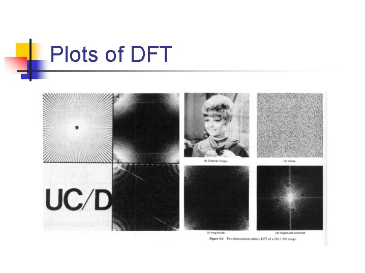
Plots of DFT

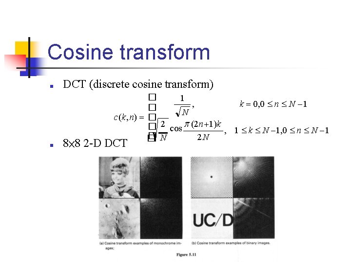
Cosine transform ■ ■ DCT (discrete cosine transform) � 1 , k 0, 0 n N 1 � N c(k, n) � � 2 cos (2 n 1)k , 1 k N 1, 0 n N 1 �N 2 N � 8× 8 2 -D DCT

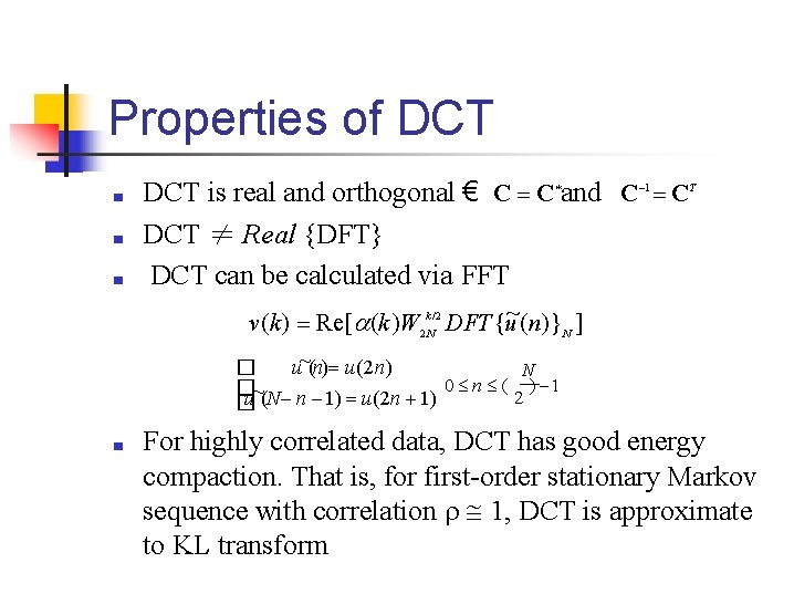
Properties of DCT ■ ■ ■ DCT is real and orthogonal € C C and C C DCT ≠ Real {DFT} DCT can be calculated via FFT * 1 T v(k ) Re[ (k )W 2 k. N/ 2 DFT{u~(n)} N ] u~(n) u(2 n) � N 0 n ( ) 1 � ~(N n 1) u(2 n 1) 2 u � ■ For highly correlated data, DCT has good energy compaction. That is, for first-order stationary Markov sequence with correlation 1, DCT is approximate to KL transform

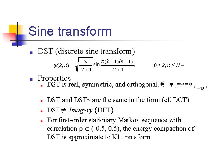
Sine transform ■ DST (discrete sine transform) (k, n) ■ Properties ■ ■ 2 (k 1)(n 1) , sin N 1 0 k, n N 1 DST is real, symmetric, and orthogonal. € ψ * ψ ψ T DST and DST-1 are the same in the form (cf. DCT) DST≠ Imagery {DFT} For first-order stationary Markov sequence with correlation (-0. 5, 0. 5), the energy compaction of DST is approximate to KL transform ψ 1

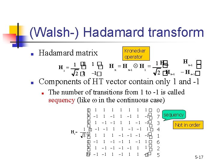
(Walsh-) Hadamard transform ■ Kronecker operator Hadamard matrix 1 1� 1 � � � H 1 2 � 1 1� ■ H n 1 � H n 1 H 1 1 � H n 1 2� H n 1 � � H n 1� Components of HT vector contain only 1 and -1 ■ The number of transitions from 1 to -1 is called sequency (like in the continuous case) H 3 1 � � 1 � 1 8� � 1� 1 1 1 1 1 1 1� 1 1� � 1 1 � 1 1� � 1 1 1 1 � � � 1 1 � 0 7 sequency 3 Not in order 4 1 6 2 5 5 -17

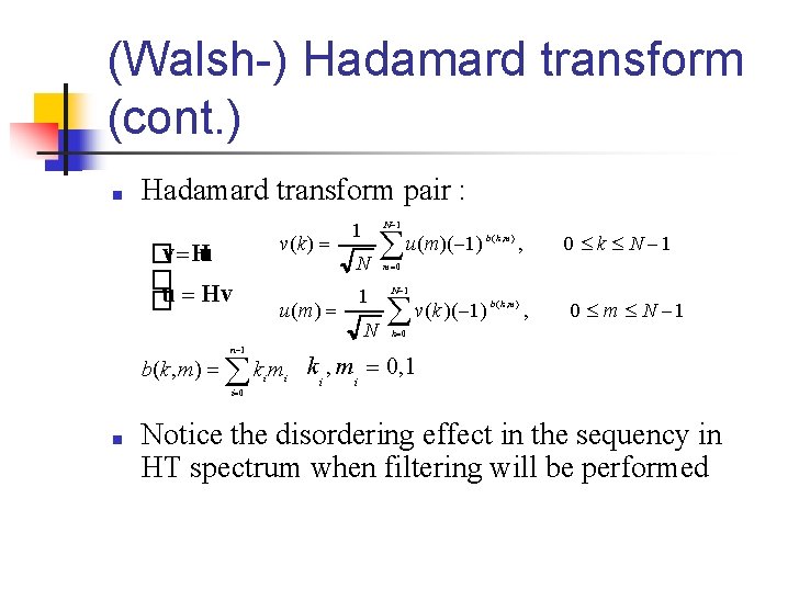
(Walsh-) Hadamard transform (cont. ) ■ Hadamard transform pair : v(k ) �v Hu � �u Hv 1 N 1 N u(m)( 1) b ( k , m ) , 0 k N 1 m 0 u(m) 1 N 1 v(k )( 1) N b ( k , m ) , 0 m N 1 k 0 b(k, m) n 1 k m i i 0 ■ i k i , mi 0, 1 Notice the disordering effect in the sequency in HT spectrum when filtering will be performed

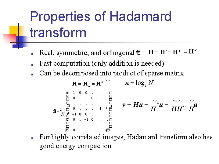
Properties of Hadamard transform ■ ■ ■ H H * H T H 1 Real, symmetric, and orthogonal € Fast computation (only addition is needed) Can be decomposed into product of sparse matrix H Hn H n 1 � � 0 � �. � ~ 10 � H 1 2� � 0 � �. � 0� � ■ 1 0 0 . ~ n log 2 N . . . � � 0 1 1 0. . . � � 0. . 1 1� 1 0 0. . � � 0 1 1 0. . . � � � 0. . 1 1� v Hu ~n ~~ ~ u . . . u H HH H For highly correlated images, Hadamard transform also has good energy compaction

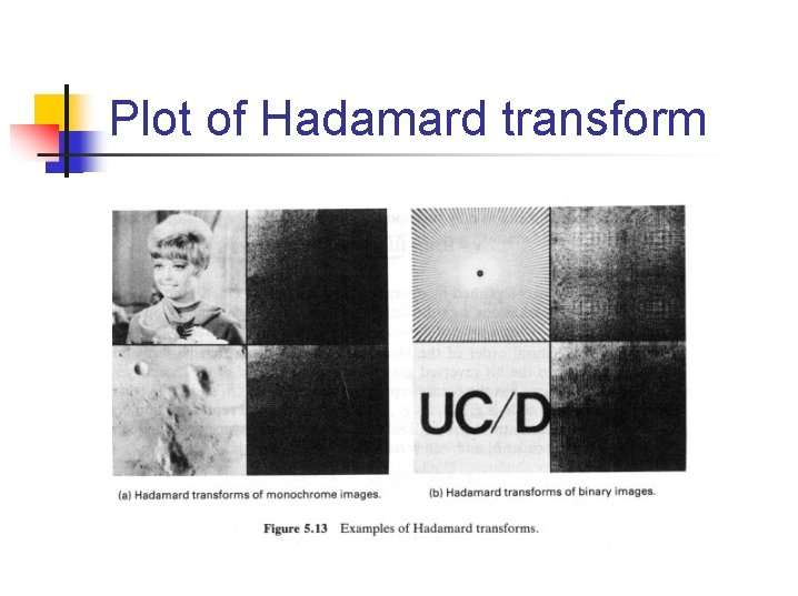
Plot of Hadamard transform

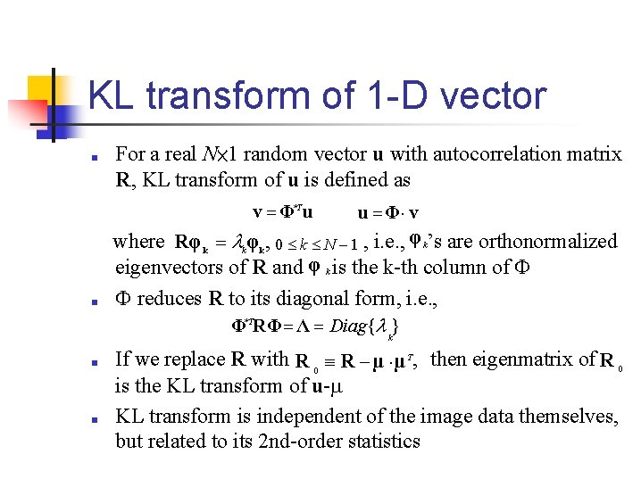
KL transform of 1 -D vector ■ For a real N× 1 random vector u with autocorrelation matrix R, KL transform of u is defined as v Φ*T u where Rφ φ , 0 k N 1 , i. e. , φ k’s are orthonormalized eigenvectors of R and φ k is the k-th column of reduces R to its diagonal form, i. e. , Φ RΦ Λ Diag{ } k ■ u Φ v k k *T k ■ ■ If we replace R with R 0 R µ µ T, then eigenmatrix of R 0 is the KL transform of u- KL transform is independent of the image data themselves, but related to its 2 nd-order statistics

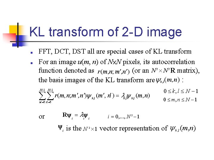
KL transform of 2 -D image ■ ■ FFT, DCT, DST all are special cases of KL transform For an image u(m, n) of N×N pixels, its autocorrelation function denoted as r(m, n; m , n ) (or an N N R matrix), the basis images of the KL transform are k , l (m, n) : 2 N 1 r(m, n; m , n ) k , l (m, n) m 0 n 0 or Rψ i iψ i 2 0 k, l N 1 0 m, n N 1 i 0, . . . , N 2 1 ψi is the N 1 vector representation of k , l (m, n) 2

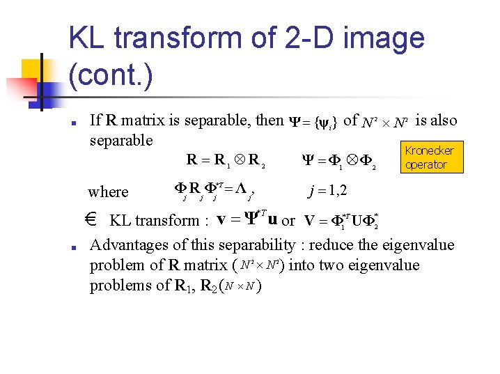
KL transform of 2 -D image (cont. ) ■ If R matrix is separable, then Ψ {ψ } of N N is also separable Kronecker R R 1 R 2 Ψ Φ 1 Φ 2 operator 2 2 i where Φj R j Φj*T Λ j, j 1, 2 € KL transform : v Ψ*T u or V Φ UΦ ■ *T * 1 2 Advantages of this separability : reduce the eigenvalue problem of R matrix ( N N ) into two eigenvalue problems of R 1, R 2 ( N N ) 2 2

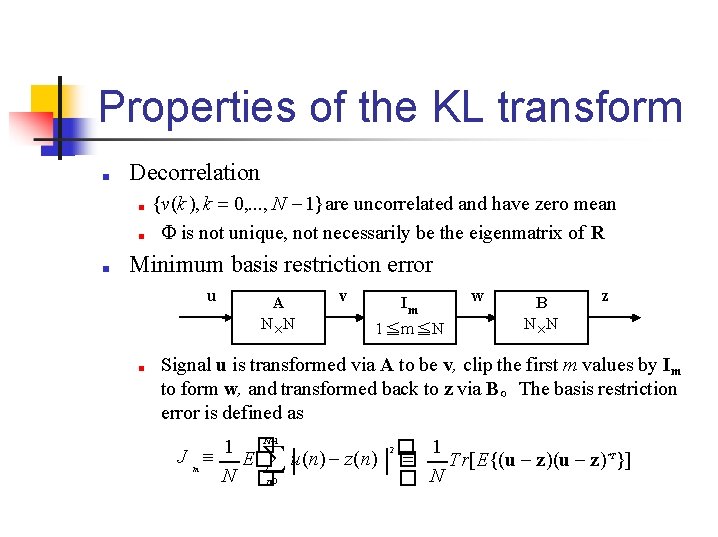
Properties of the KL transform ■ Decorrelation ■ ■ ■ {v(k ), k 0, . . . , N 1} are uncorrelated and have zero mean is not unique, not necessarily be the eigenmatrix of R Minimum basis restriction error u ■ A N N v Im 1≦m≦N w B N N z Signal u is transformed via A to be v, clip the first m values by Im to form w, and transformed back to z via B。The basis restriction error is defined as N 1 � 2 1 1 J m E� u(n) z(n) � � Tr[E{(u z)*T}] N �n 0 � N

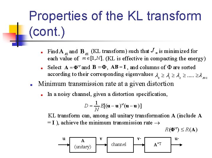
Properties of the KL transform (cont. ) ■ ■ ■ Find A KL and B KL (KL transform) such that J m is minimized for each value of m [1, N ]. (KL is effective in compacting the energy) Select A Φ*T and B Φ , AB I , and columns of are sorted according to their corresponding eigenvalues . . . 0 1 2 N 1 Minimum transmission rate at a given distortion ■ In a noisy channel, given a distortion specification, D 1 E[(u u. )*T (u u. )] N KL transform can, among all unitary transformation A (include A = I ), achieve the minimum transmission rate R(Φ*T ) R(A) u A (unitary) v. v channel u. A*T

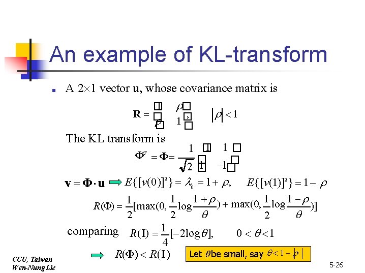
An example of KL-transform ■ A 2 1 vector u, whose covariance matrix is 1 � � , 1 R � � � 1 � The KL transform is Φ Φ *T 1 1� 1 � � � 1 1� 2� E{[v(0)]2} 0 1 , E{[v(1)]2 } 1 1 1 ) max(0, 1 log 1 1 R(Φ) [max(0, log )] 2 2 2 comparing R(I) 1 [ 2 log ], 0 1 4 Let be small, say 1 R(Φ) R(I) v Φ u CCU, Taiwan Wen-Nung Lie 5 -26

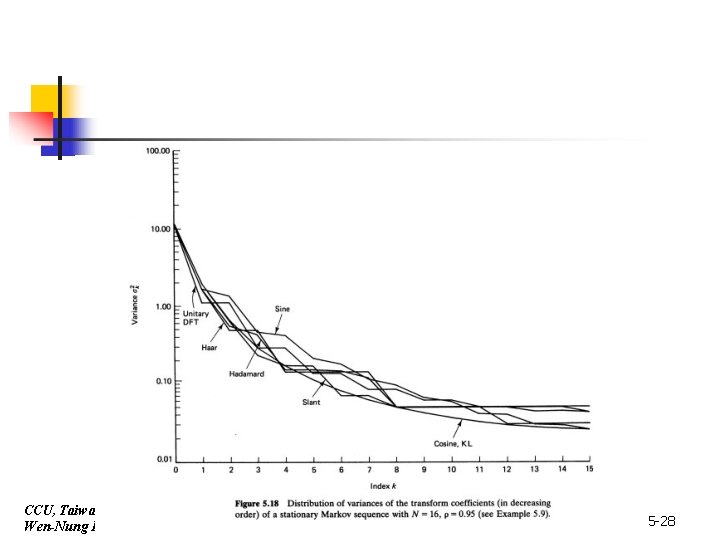
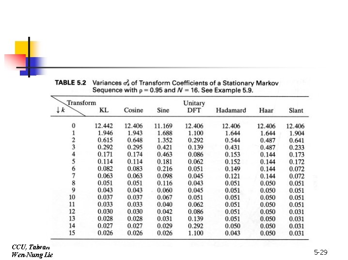
Comparison of energy distribution between transforms ■ ■ ■ CCU, Taiwan Wen-Nung Lie For first-order stationary Markov process with large , DCT is comparable to KL With small , DST is comparable to KL For any , we can find a faster sinusoidal transform (DCT or DST) to substitute for the optimal KL transform which needs covariance matrix to compute transform basis vectors 5 -27

CCU, Taiw an Wen-Nung Lie 5 -28

CCU, Taiwan Wen-Nung Lie 5 -29

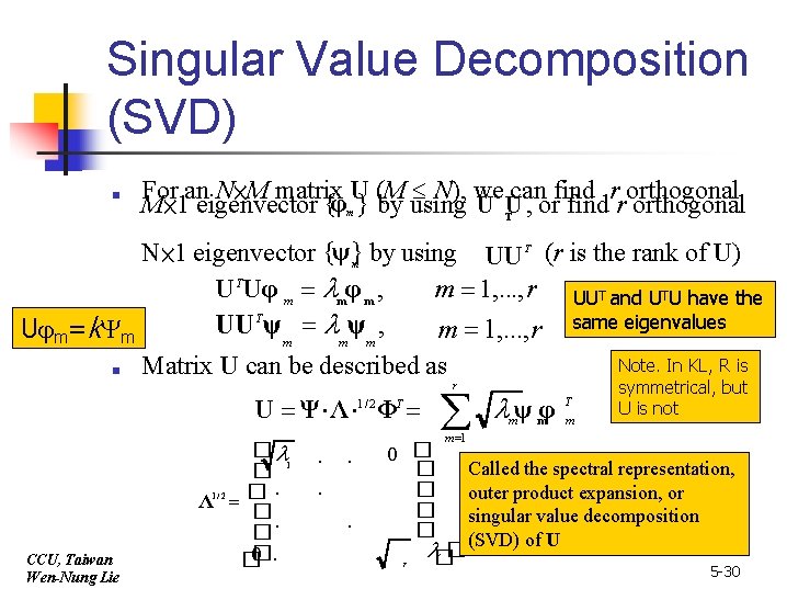
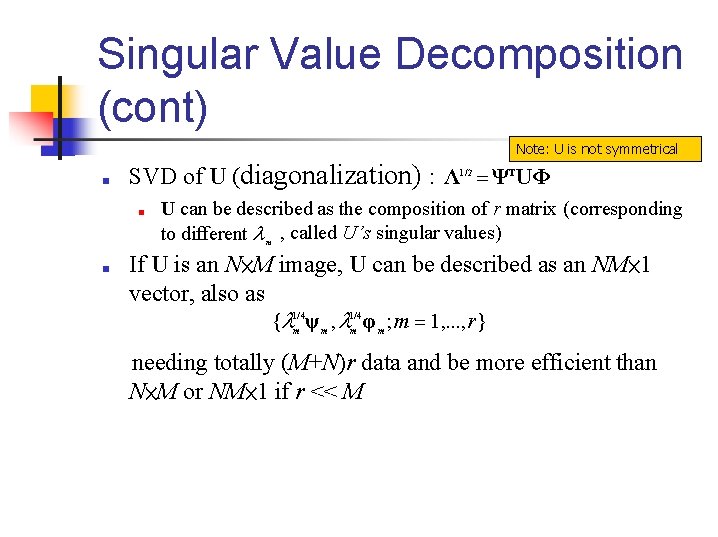
Singular Value Decomposition (SVD) ■ For an N×M matrix U (M N), we can find r orthogonal M× 1 eigenvector {φm } by using U TU , or find r orthogonal N× 1 eigenvector {ψ}m by using UU T (r is the rank of U) UTUφ m mφ m , m 1, . . . , r UUT and UTU have the UU Tψ m mψ m , m 1, . . . , r same eigenvalues U m=k m Note. In KL, R is ■ Matrix U can be described as U Ψ Λ Φ 1/ 2 CCU, Taiwan Wen-Nung Lie � � 1. Λ 1/ 2 � �. � 0 . . T r ψφ m m T m symmetrical, but U is not m 1 0 � � Called the spectral representation, � outer product expansion, or � singular value decomposition � (SVD) of U �� r 5 -30

Singular Value Decomposition (cont) Note: U is not symmetrical ■ SVD of U (diagonalization) : Λ Ψ UΦ 1/ 2 ■ ■ T U can be described as the composition of r matrix (corresponding to different m , called U’s singular values) If U is an N×M image, U can be described as an NM× 1 vector, also as { ψ , φ ; m 1, . . . , r} 1/ 4 m m m needing totally (M+N)r data and be more efficient than N×M or NM× 1 if r << M

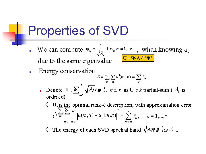
Properties of SVD ■ We can compute ψm 1 Uφ m, m 1, . . . r m ■ , when knowing φ m U Ψ Λ 1/ 2 ΦT due to the same eigenvalue Energy conservation E u (m, n) 2 m m k ■ n m mψ mφ m , k r, as U’s k partial-sum ( m is Denote U k m 1 ordered) € U k is the optimal rank-k description, with approximation error T k 2 M m 1 N n 1 2 u(m, n) u k (m, n) r , m k 1, . . . , r m k 1 € The energy of each SVD spectral band ψ φ is T m m

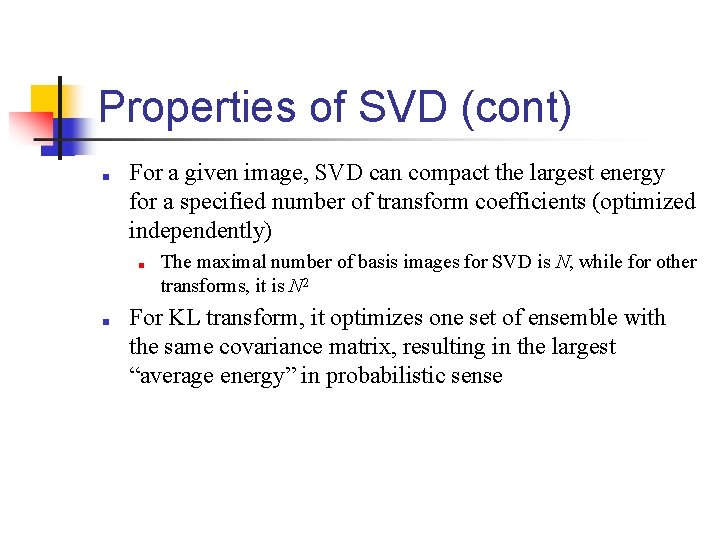
Properties of SVD (cont) ■ For a given image, SVD can compact the largest energy for a specified number of transform coefficients (optimized independently) ■ ■ The maximal number of basis images for SVD is N, while for other transforms, it is N 2 For KL transform, it optimizes one set of ensemble with the same covariance matrix, resulting in the largest “average energy” in probabilistic sense