Fundamentals of EMC Time Domain vs Frequency Domain


 l Equipment n Tektronix MDO")
 7")
 8")
 9")


/x (next slide) NOTE:")
/x Response of |sin(x)/x|: 0 for x = nπ 1/x")


; τr = τf = 40 ns 2")
; τr = τf = 360 ns 2")
; τr = τf = 10 µs 2")
; τr = τf = 40 ns 2")
; τr = τf = 360 ns 2")
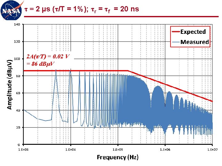
; τr = τf = 40 ns 2")
; τr = τf = 350 ns 2")
; τr = τf = 160 ns 2")
; τr = τf = 400 ns 2")
; τr = τf = 8 ns")
 l Measured spectra show good agreement with expected values n")
 l Signal spectra significantly more determined by rise/fall times than")
- Slides: 37
Fundamentals of EMC Time Domain vs. Frequency Domain John Mc. Closkey NASA/GSFC Chief EMC Engineer Code 565 Building 23, room E 203 301 -286 -5498 John. C. Mc. Closkey@nasa. gov 1
Full Demo/Tutorial Video of full demonstration/tutorial on NESC Academy website n “Effects of Rise/Fall Times on Signal Spectra” n Link on GSFC EMC Working Group XSPACES SITE: • https: //xspaces. gsfc. nasa. gov/display/EMCWG/Home 2
Purpose of Demo/Tutorial l Demonstrate the relationship between time domain and frequency domain representations of signals l In particular, demonstrate the relationship between rise/fall times of digital clock-type signals and their associated spectra l Fast rise/fall times can produce significant high frequency content out to 1000 th harmonic and beyond n Common cause of radiated emissions that can interfere with on-board receivers n Can be reduced by limiting rise/fall times 3
Topics l Sinusoid: Time Domain vs. Frequency Domain l Fourier series expansions of: n Square wave n Rectangular pulse train n Trapezoidal waveform l Comparison to measured results for these waveforms l Observations 4
Demo 4: Time Domain vs. Frequency Domain 5
Demo 4: Time Domain vs. Frequency Domain (cont. ) l Equipment n Tektronix MDO 3104 oscilloscope (built-in signal generator) n 2 RG-58 coax cables n T connector n BNC-N adaptor l Setup n AFG: 1 MHz sine, square, pulse with 300 ns width (30% duty cycle) 6
Demo 4: Time Domain vs. Frequency Domain (cont. ) 7
Demo 4: Time Domain vs. Frequency Domain (cont. ) 8
Demo 4: Time Domain vs. Frequency Domain (cont. ) 9
Sinusoid: Time Domain vs. Frequency Domain TIME DOMAIN FREQUENCY DOMAIN Amplitude A f Frequency 10
Fourier Series Expansion of Signal Waveforms l Recommended reading for an in-depth look at Fourier series expansions of signal waveforms: n Clayton Paul, “Introduction to Electromagnetic Compatibility, ” sections 3. 1 and 3. 2 11
Fourier Series Expansion of Square Wave Odd harmonics only 12
Fourier Series Expansion of Rectangular Pulse Train Even harmonics included sin(x)/x (next slide) NOTE: For 50% duty cycle (τ/T = 0. 5), this equation reduces to that for the square wave on the previous slide. 13
Response and Envelope of sin(x)/x Response of |sin(x)/x|: 0 for x = nπ 1/x for x = (n+1)π/2 Envelope of |sin(x)/x|: 1 for x < 1 1/x for x > 1 Lines meet at x = 1 14
Envelope of Rectangular Pulse Train Spectrum DC offset Low frequency “plateau” Harmonic response 0 d. B/decade -20 d. B/ dec ade etc… f 1 PULSE WIDTH f 2 f 3 f 4 f 5 f 15
Fourier Series Expansion of Trapezoidal Waveform A τr τ T τf NOTE: τr and τf are generally measured between 10% and 90% of the minimum and maximum values of the waveform. Assume τr = τf : Additional sin(x)/x term due to rise/fall time 16
Envelope of Trapezoidal Waveform Spectrum DC offset Low frequency “plateau” 0 d. B/decade Harmonic response (pulse width) -20 d. B/ Harmonic response (rise/fall time) dec ade -4 0 d. B /d e ca de etc… f 1 PULSE WIDTH f 2 f 3 f 4 RISE/FALL TIME f 5 f 17
Envelope of Trapezoidal Waveform Spectrum Slower rise/fall times provide additional roll-off of higher order harmonics 0 d. B/decade -20 d. B/ dec ade -4 0 d. B /d e ca de f PULSE WIDTH RISE/FALL TIME 18
Time Domain vs. Frequency Domain Test Setup WAVETEK 801 pulse generator TEKTRONIX RSA 5103 A spectrum analyzer (50 Ω input) TEKTRONIX DPO 7054 oscilloscope (1 MΩ input) 19
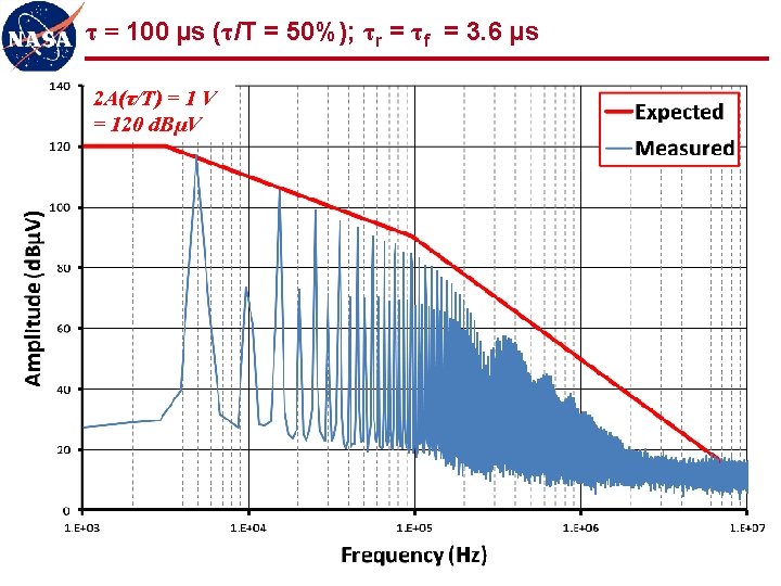
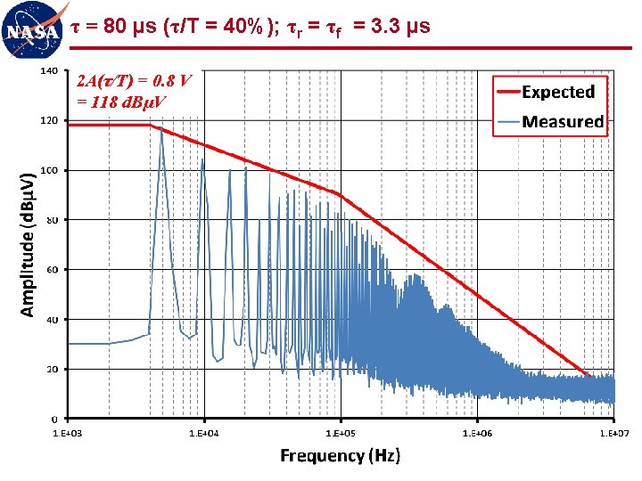
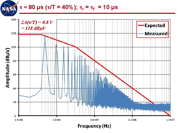
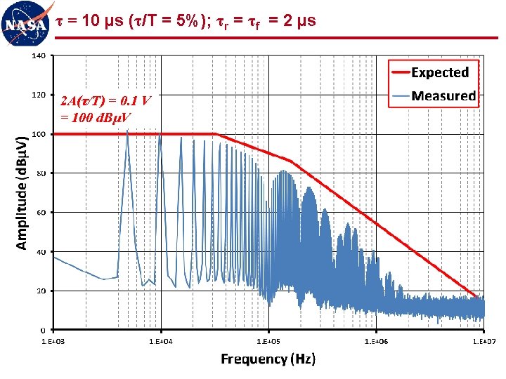
Applied Waveform A τr τ T τf A=1 V T = 200 µs (f 0 = 5 k. Hz) τ, τr , & τf varied as indicated on following slides 20
τ = 100 µs (τ/T = 50%); τr = τf = 40 ns 2 A(τ/T) = 1 V = 120 d. BµV 21
τ = 100 µs (τ/T = 50%); τr = τf = 360 ns 2 A(τ/T) = 1 V = 120 d. BµV 22
τ = 100 µs (τ/T = 50%); τr = τf = 10 µs 2 A(τ/T) = 1 V = 120 d. BµV 24
τ = 80 µs (τ/T = 40%); τr = τf = 40 ns 2 A(τ/T) = 0. 8 V = 118 d. BµV 25
τ = 80 µs (τ/T = 40%); τr = τf = 360 ns 2 A(τ/T) = 0. 8 V = 118 d. BµV 26
τ = 10 µs (τ/T = 5%); τr = τf = 40 ns 2 A(τ/T) = 0. 1 V = 100 d. BµV 29
τ = 10 µs (τ/T = 5%); τr = τf = 350 ns 2 A(τ/T) = 0. 1 V = 100 d. BµV 30
τ = 2 µs (τ/T = 1%); τr = τf = 160 ns 2 A(τ/T) = 0. 02 V = 86 d. BµV 33
τ = 2 µs (τ/T = 1%); τr = τf = 400 ns 2 A(τ/T) = 0. 02 V = 86 d. BµV 34
τ = 100 ns (τ/T = 0. 05%); τr = τf = 8 ns 2 A(τ/T) = 0. 001 V = 60 d. BµV 35
Observations (1 of 2) l Measured spectra show good agreement with expected values n “ 3 -line” envelope provides simple, accurate, and powerful analytical tool for correlating signal spectra to trapezoidal waveforms l Even harmonics n Reduced, but not zero, amplitude for 50% duty cycle n Varying amplitude for other than 50% duty cycle n Must be considered as potentially significant contributors to spectrum l Low frequency plateau scales with duty cycle n Spectrum for low duty cycle waveforms gives artificial indication of low amplitude n First “knee” frequency may be quite high, producing relatively flat spectrum for many harmonics (100 s or 1000 s in these examples) n Low duty cycle waveforms should be observed in time domain (oscilloscope) as well as frequency domain (spectrum analyzer) 36
Observations (2 of 2) l Signal spectra significantly more determined by rise/fall times than by fundamental frequency of waveform l Uncontrolled rise/fall times can produce significant frequency content out to 1000 th harmonic and beyond n Common cause of radiated emissions n 5 MHz clock can easily produce harmonics out to 5 GHz and beyond n Potential interference to S-band receiver (~2 GHz), GPS (~1. 5 GHz), etc. l Controlling rise/fall times can significantly limit high frequency content at source LIMIT THOSE RISE/FALL TIMES!!! 37