Frequency domain Image Processing Comp 344 Tutorial Kai

Frequency domain Image Processing Comp 344 Tutorial Kai Zhang

Outline n Matlab preliminaries n Matlab function design n Shifting frequency component n Low pass filtering design

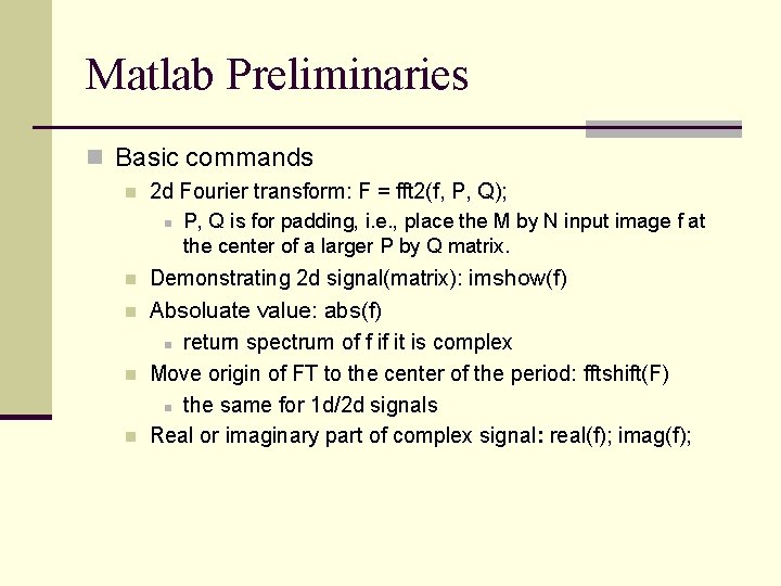
Matlab Preliminaries n Basic commands n 2 d Fourier transform: F = fft 2(f, P, Q); n P, Q is for padding, i. e. , place the M by N input image f at the center of a larger P by Q matrix. n Demonstrating 2 d signal(matrix): imshow(f) n Absoluate value: abs(f) n return spectrum of f if it is complex Move origin of FT to the center of the period: fftshift(F) n the same for 1 d/2 d signals Real or imaginary part of complex signal: real(f); imag(f); n n

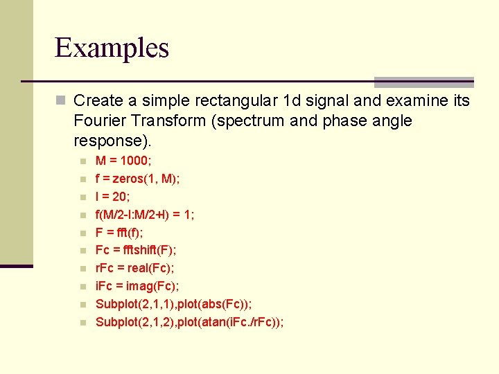
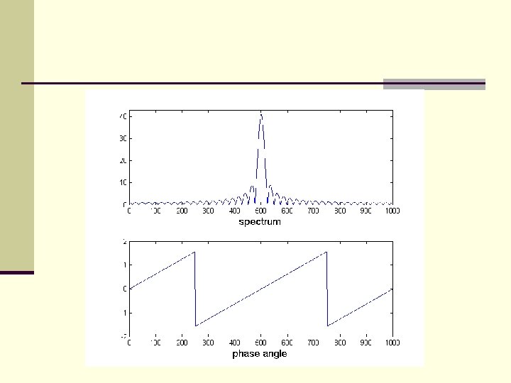
Examples n Create a simple rectangular 1 d signal and examine its Fourier Transform (spectrum and phase angle response). n n n n n M = 1000; f = zeros(1, M); l = 20; f(M/2 -l: M/2+l) = 1; F = fft(f); Fc = fftshift(F); r. Fc = real(Fc); i. Fc = imag(Fc); Subplot(2, 1, 1), plot(abs(Fc)); Subplot(2, 1, 2), plot(atan(i. Fc. /r. Fc));

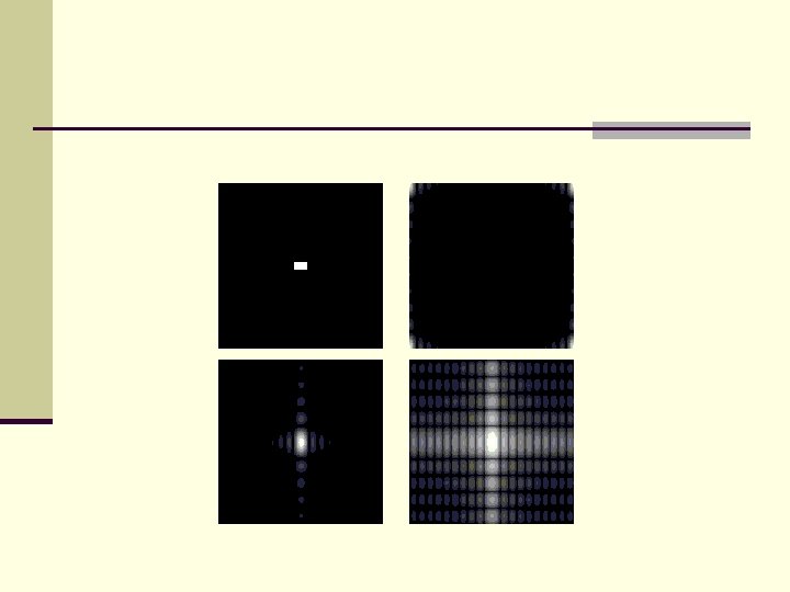
Examples n Examine the fourier transform of a synthetic image n n n f = ones(10, 20); F = fft 2(f, 500); f 1 = zeros(500, 500); f 1(240: 260, 230: 270) = 1; subplot(2, 2, 1); imshow(f 1, []); S = abs(F); subplot(2, 2, 2); imshow(S, []); Fc = fftshift(F); S 1 = abs(Fc); subplot(2, 2, 3); imshow(S 1, []); S 2 = log(1+S 1); subplot(2, 2, 4); imshow(S 2, []);

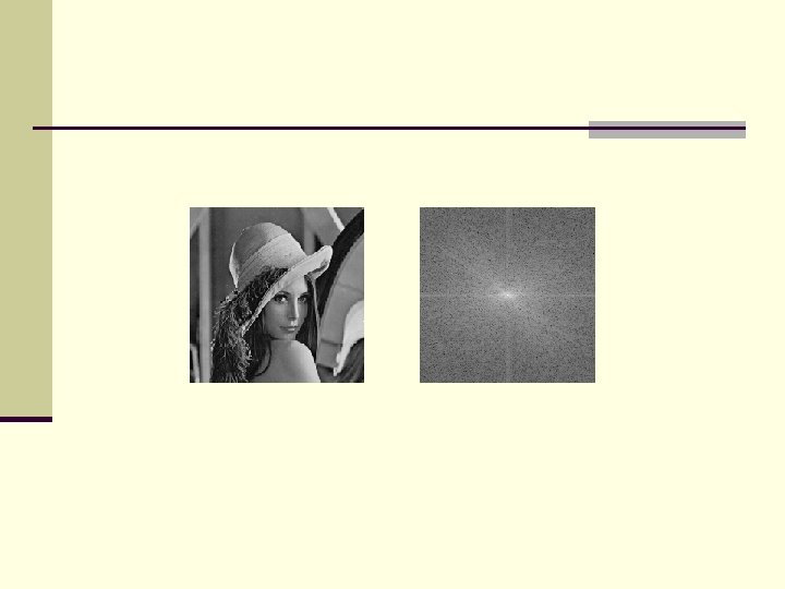
Example n Fourier transform of natural images n f = imread(‘lenna. jpg’); n subplot(1, 2, 1), imshow(f); n f = double(f); n F = fft 2(f); n Fc = fftshift(F); n S = log(1+abs(Fc)); n Subplot(1, 2, 2), imshow(S, []);

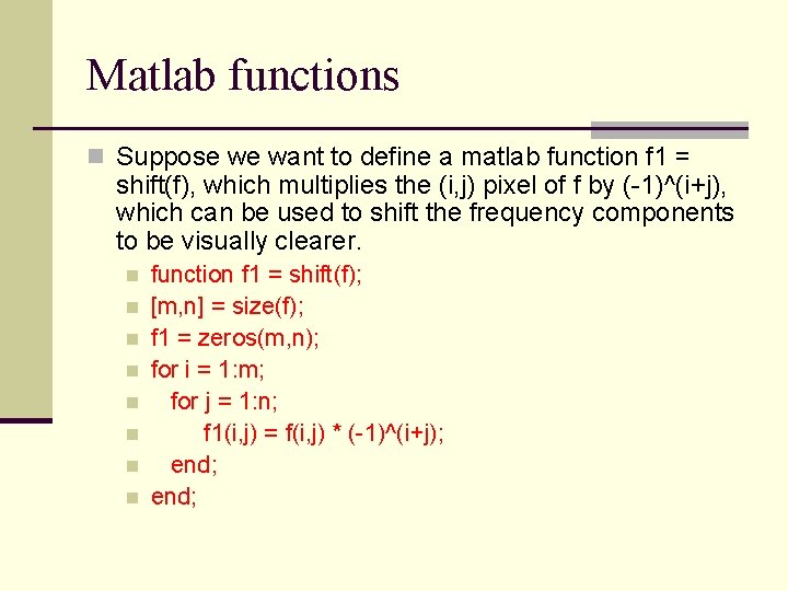
Matlab functions n Suppose we want to define a matlab function f 1 = shift(f), which multiplies the (i, j) pixel of f by (-1)^(i+j), which can be used to shift the frequency components to be visually clearer. n n n n function f 1 = shift(f); [m, n] = size(f); f 1 = zeros(m, n); for i = 1: m; for j = 1: n; f 1(i, j) = f(i, j) * (-1)^(i+j); end;

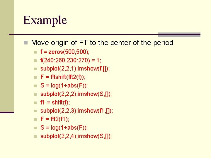
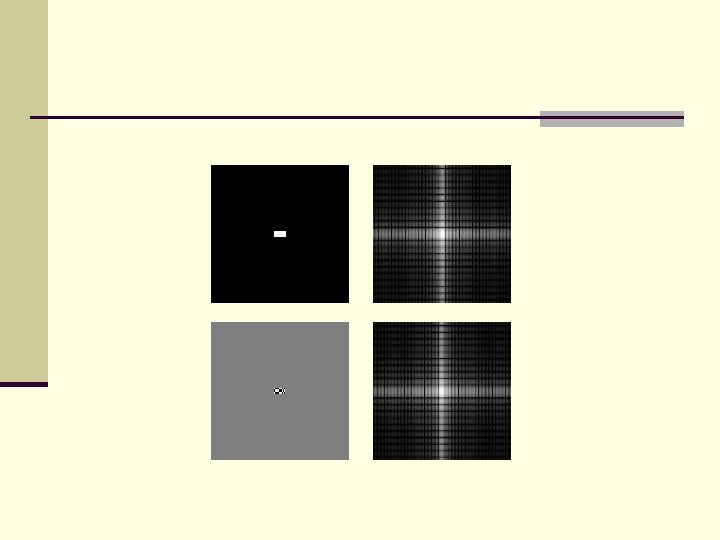
Example n Move origin of FT to the center of the period n n n f = zeros(500, 500); f(240: 260, 230: 270) = 1; subplot(2, 2, 1); imshow(f, []); F = fftshift(fft 2(f)); S = log(1+abs(F)); subplot(2, 2, 2); imshow(S, []); f 1 = shift(f); subplot(2, 2, 3); imshow(f 1, []); F = fft 2(f 1); S = log(1+abs(F)); subplot(2, 2, 4); imshow(S, []);

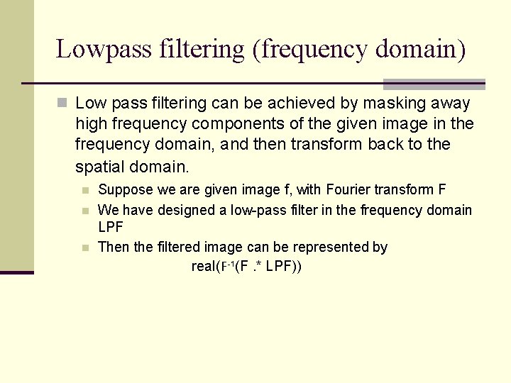
Lowpass filtering (frequency domain) n Low pass filtering can be achieved by masking away high frequency components of the given image in the frequency domain, and then transform back to the spatial domain. n n n Suppose we are given image f, with Fourier transform F We have designed a low-pass filter in the frequency domain LPF Then the filtered image can be represented by real(F-1(F. * LPF))

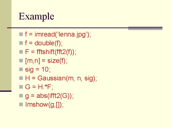
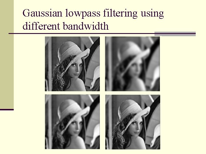
Example n n n n n f = imread(‘lenna. jpg’); f = double(f); F = fftshift(fft 2(f)); [m, n] = size(f); sig = 10; H = Gaussian(m, n, sig); G = H. *F; g = abs(ifft 2(G)); Imshow(g, []);

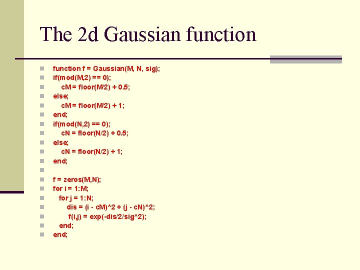
The 2 d Gaussian function n n n n function f = Gaussian(M, N, sig); if(mod(M, 2) == 0); c. M = floor(M/2) + 0. 5; else; c. M = floor(M/2) + 1; end; if(mod(N, 2) == 0); c. N = floor(N/2) + 0. 5; else; c. N = floor(N/2) + 1; end; f = zeros(M, N); for i = 1: M; for j = 1: N; dis = (i - c. M)^2 + (j - c. N)^2; f(i, j) = exp(-dis/2/sig^2); end;

Gaussian lowpass filtering using different bandwidth