The ERP Boot Camp Filtering and Linear Systems
The ERP Boot Camp Filtering and Linear Systems Analysis All slides © S. J. Luck, except as indicated in the notes sections of individual slides Slides may be used for nonprofit educational purposes if this copyright notice is included, except as noted Permission must be obtained from the copyright holder(s) for any other use
Filtering Overview • Filter- To remove some components of an input and pass others - We will concentrate on Finite Impulse Response (FIR) filters • Different approaches to filtering - • Hardware filters Filtering by conversion to frequency domain Filtering by computing weighted average of adjacent points Filtering by convolving with impulse response function These are all mathematically equivalent - Relatively simple relationships between them • By understanding these relationships, you will have a much deeper understanding of the nature of ERPs - But this stuff can blow your mind…
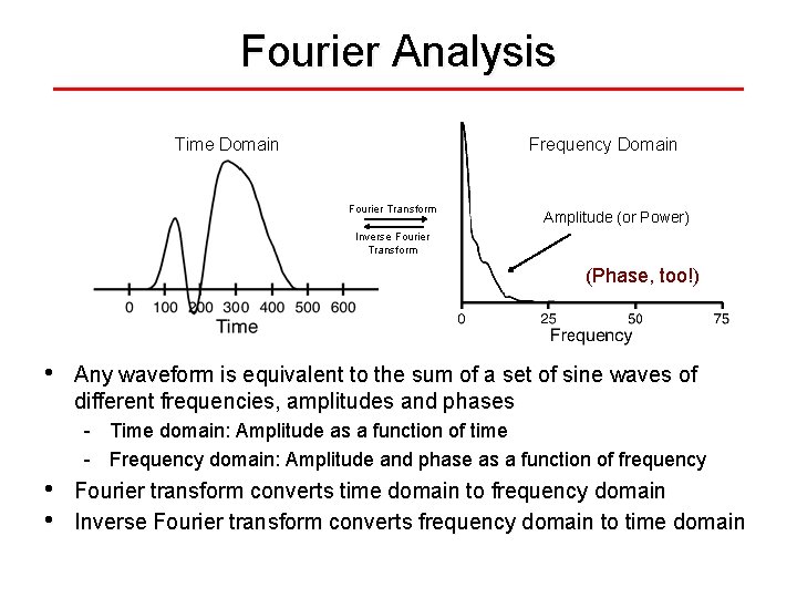
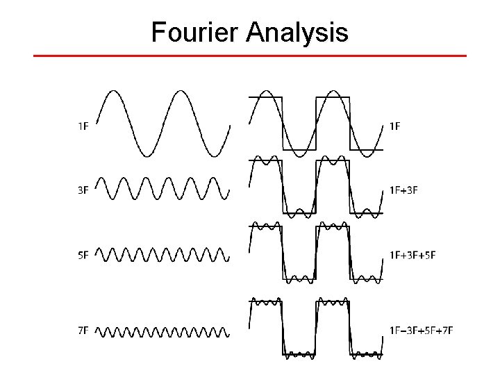
Fourier Analysis Time Domain Frequency Domain Fourier Transform Amplitude (or Power) Inverse Fourier Transform (Phase, too!) • Any waveform is equivalent to the sum of a set of sine waves of different frequencies, amplitudes and phases - Time domain: Amplitude as a function of time - Frequency domain: Amplitude and phase as a function of frequency • • Fourier transform converts time domain to frequency domain Inverse Fourier transform converts frequency domain to time domain
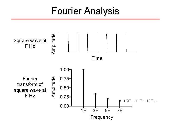
Square wave at F Hz Amplitude Fourier Analysis Fourier transform of square wave at F Hz Amplitude Time + 9 F + 11 F + 13 F … Frequency
Fourier Analysis
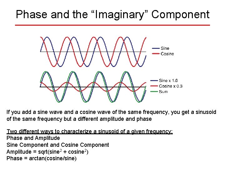
Phase and the “Imaginary” Component If you add a sine wave and a cosine wave of the same frequency, you get a sinusoid of the same frequency but a different amplitude and phase Two different ways to characterize a sinusoid of a given frequency: Phase and Amplitude Sine Component and Cosine Component Amplitude = sqrt(sine 2 + cosine 2) Phase = arctan(cosine/sine)
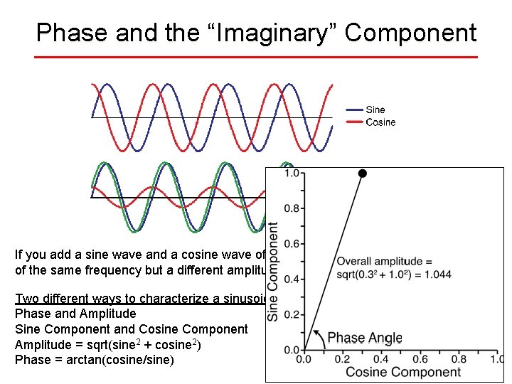
Phase and the “Imaginary” Component If you add a sine wave and a cosine wave of the same frequency, you get a sinusoid of the same frequency but a different amplitude and phase Two different ways to characterize a sinusoid of a given frequency: Phase and Amplitude Sine Component and Cosine Component Amplitude = sqrt(sine 2 + cosine 2) Phase = arctan(cosine/sine)
Fundamental Principle #1 • Power at a frequency in a Fourier transform does not mean that an oscillation was present at that frequency - What the #$%$#&@? !!! - Then what does power at a frequency mean? • Power at a frequency means that a sine wave at that frequency, when added to other sine waves at other frequencies, can create an equivalent waveform - It does not mean that the biological signal consists of the sum of these sine waves
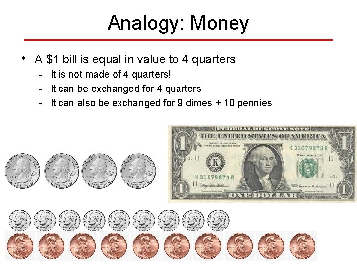
Analogy: Money • A $1 bill is equal in value to 4 quarters - It is not made of 4 quarters! - It can be exchanged for 4 quarters - It can also be exchanged for 9 dimes + 10 pennies
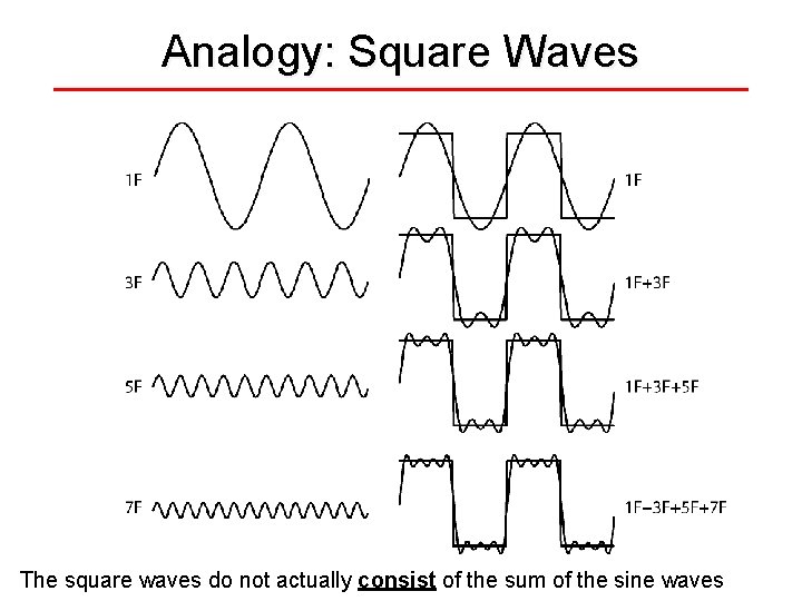
Analogy: Square Waves The square waves do not actually consist of the sum of the sine waves
Basis Functions In mathematics, there are many sets of “basis functions” that can be used to recreate a given set of data • • • Sine waves Polynomials (X 0, X 1, X 2, X 3, …) Spline functions PCA ICA Any waveform can be reconstructed in any of these ways, and there is no underlying “truth” to the reconstructions
Nonetheless… • Bona fide oscillations are sometimes present - 60 -Hz line noise - Alpha - Gamma oscillations have been clearly demonstrated in animals • Noise is often largely confined to distinct frequency bands - Skin potentials (almost entirely below 1 Hz) - Muscle noise (almost entirely above 20 Hz) • • Time-frequency analyses can reveal brain activity that is invisible in conventional averages It is still useful to think in terms of the frequency domain, as long as you’re careful
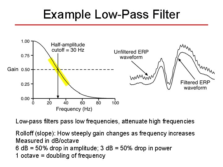
Example Low-Pass Filter Low-pass filters pass low frequencies, attenuate high frequencies Rolloff (slope): How steeply gain changes as frequency increases Measured in d. B/octave 6 d. B = 50% drop in amplitude; 3 d. B = 50% drop in power 1 octave = doubling of frequency
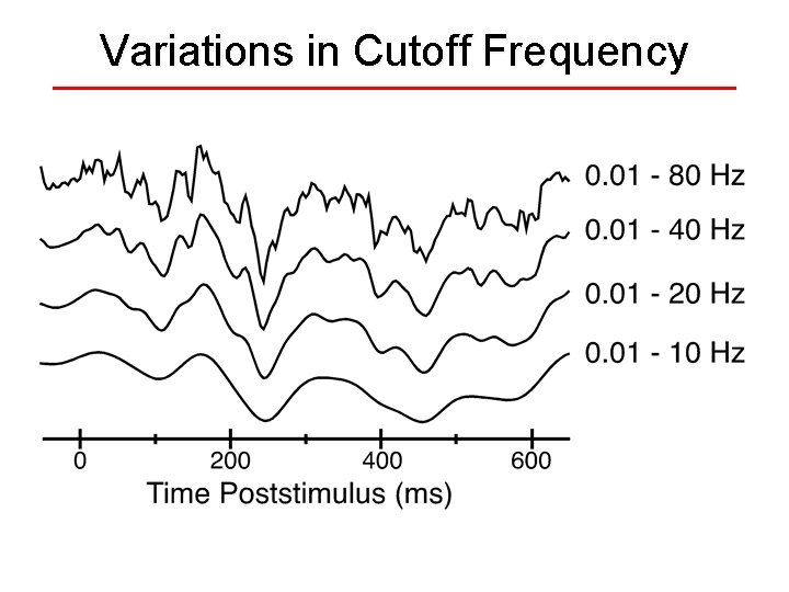
Variations in Cutoff Frequency
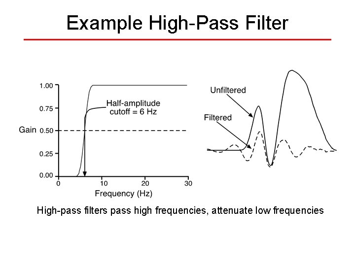
Example High-Pass Filter High-pass filters pass high frequencies, attenuate low frequencies
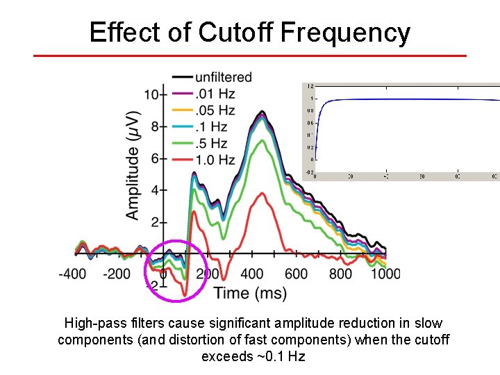
Effect of Cutoff Frequency High-pass filters cause significant amplitude reduction in slow components (and distortion of fast components) when the cutoff exceeds ~0. 1 Hz
Why are filters necessary? • Nyquist Theorem - Need to make sure we don’t have frequencies >= 1/2 the sampling rate • Noise reduction - • • Low-pass filters for muscle noise High-pass filters for skin potentials Notch filters for 50/60 -Hz line noise But filters distort your data, so they should be used sparingly Hansen’s axiom: There is no substitute for clean data
Fundamental Principle #2 • Precision (spread) in frequency domain is inversely related to precision (spread) in time domain - What is the time domain representation of an infinitesimally narrow spike in frequency domain? - What is the frequency domain representation of an instantaneous impulse in the time domain? • • • The more you filter, the more temporal precision you lose The sharper your filter rolloffs, the more temporal precision you lose The loss of temporal precision can create artifacts that will lead to incorrect conclusions
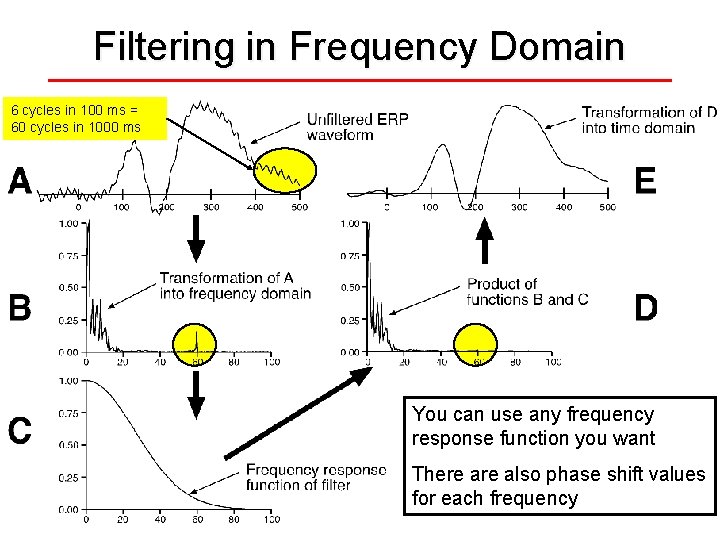
Filtering in Frequency Domain 6 cycles in 100 ms = 60 cycles in 1000 ms You can use any frequency response function you want There also phase shift values for each frequency
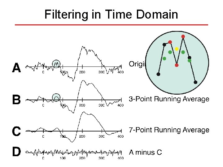
Filtering in Time Domain
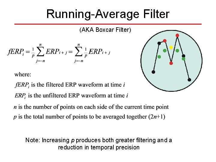
Running-Average Filter (AKA Boxcar Filter) Note: Increasing p produces both greater filtering and a reduction in temporal precision
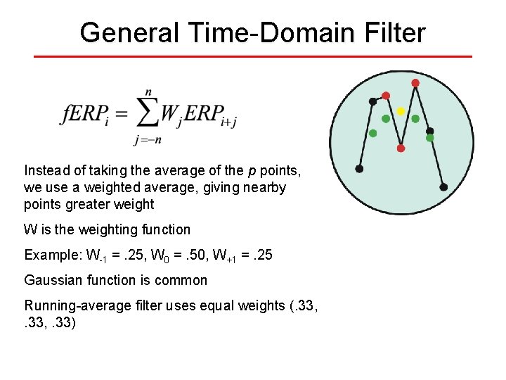
General Time-Domain Filter Instead of taking the average of the p points, we use a weighted average, giving nearby points greater weight W is the weighting function Example: W-1 =. 25, W 0 =. 50, W+1 =. 25 Gaussian function is common Running-average filter uses equal weights (. 33, . 33)
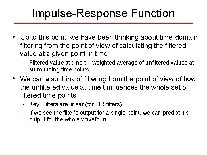
Impulse-Response Function • Up to this point, we have been thinking about time-domain filtering from the point of view of calculating the filtered value at a given point in time - Filtered value at time t = weighted average of unfiltered values at surrounding time points • We can also think of filtering from the point of view of how the unfiltered value at time t influences the whole set of filtered time points - Key: Filters are linear (for FIR filters) - If we see the filter’s output for a single point, we can predict it’s output for the whole waveform
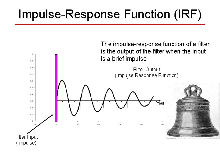
Impulse-Response Function (IRF) The impulse-response function of a filter is the output of the filter when the input is a brief impulse Filter Output (Impulse Response Function) Filter Input (Impulse)
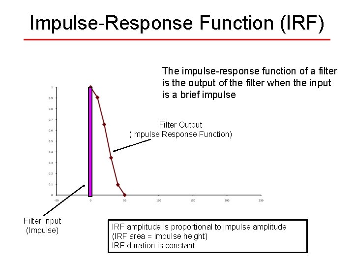
Impulse-Response Function (IRF) The impulse-response function of a filter is the output of the filter when the input is a brief impulse Filter Output (Impulse Response Function) Filter Input (Impulse) IRF amplitude is proportional to impulse amplitude (IRF area = impulse height) IRF duration is constant
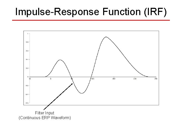
Impulse-Response Function (IRF) Filter Input (Continuous ERP Waveform)
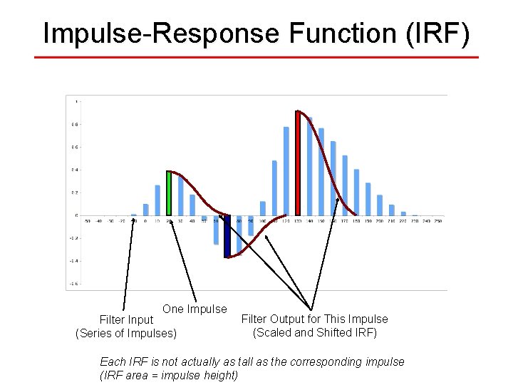
Impulse-Response Function (IRF) One Impulse Filter Input (Series of Impulses) Filter Output for This Impulse (Scaled and Shifted IRF) Each IRF is not actually as tall as the corresponding impulse (IRF area = impulse height)
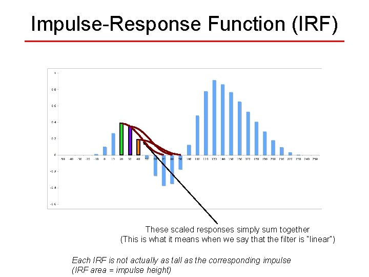
Impulse-Response Function (IRF) These scaled responses simply sum together (This is what it means when we say that the filter is “linear”) Each IRF is not actually as tall as the corresponding impulse (IRF area = impulse height)
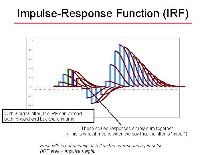
Impulse-Response Function (IRF) With a digital filter, the IRF can extend both forward and backward in time These scaled responses simply sum together (This is what it means when we say that the filter is “linear”) Each IRF is not actually as tall as the corresponding impulse (IRF area = impulse height)
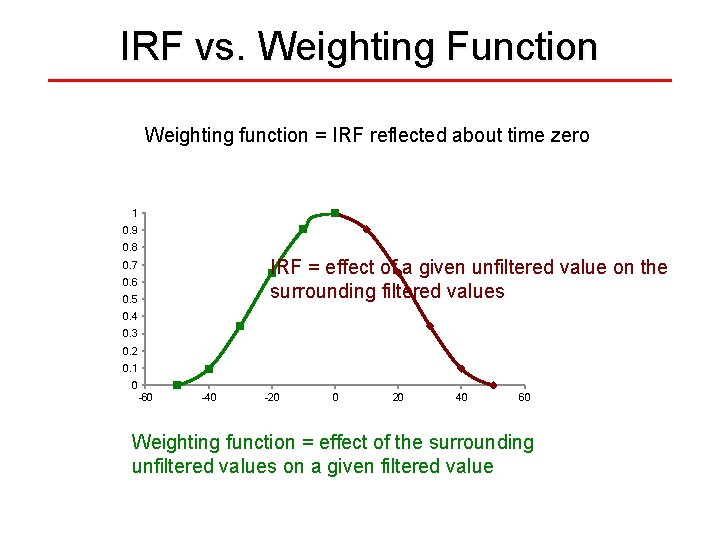
IRF vs. Weighting Function Weighting function = IRF reflected about time zero 1 0. 9 0. 8 IRF = effect of a given unfiltered value on the surrounding filtered values 0. 7 0. 6 0. 5 0. 4 0. 3 0. 2 0. 1 0 -60 -40 -20 0 20 40 60 Weighting function = effect of the surrounding unfiltered values on a given filtered value
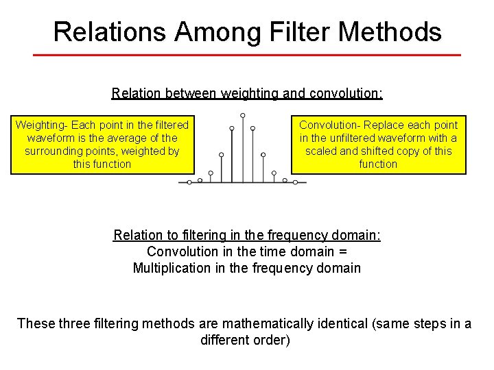
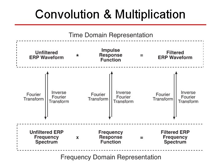
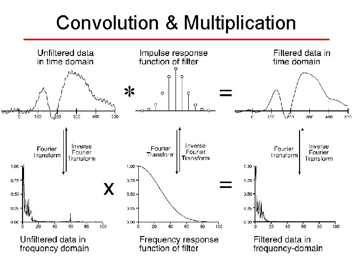
Relations Among Filter Methods Relation between weighting and convolution: Weighting- Each point in the filtered waveform is the average of the surrounding points, weighted by this function Convolution- Replace each point in the unfiltered waveform with a scaled and shifted copy of this function Relation to filtering in the frequency domain: Convolution in the time domain = Multiplication in the frequency domain These three filtering methods are mathematically identical (same steps in a different order)
Convolution & Multiplication
Convolution & Multiplication
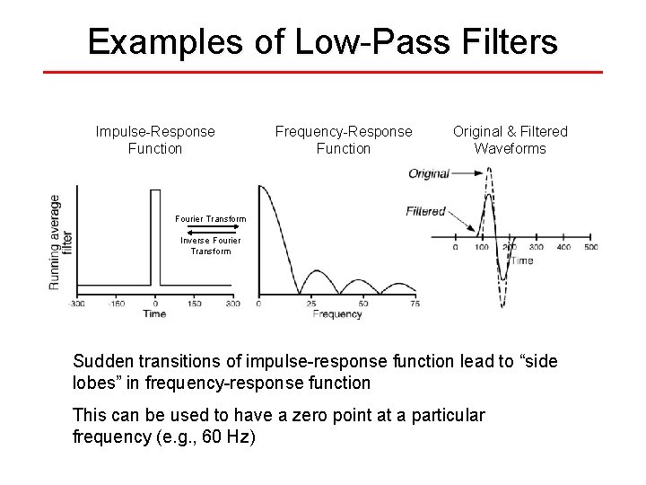
Examples of Low-Pass Filters Impulse-Response Function Frequency-Response Function Original & Filtered Waveforms Fourier Transform Inverse Fourier Transform Sudden transitions of impulse-response function lead to “side lobes” in frequency-response function This can be used to have a zero point at a particular frequency (e. g. , 60 Hz)
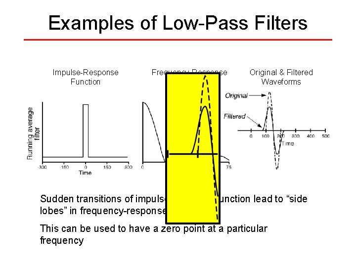
Examples of Low-Pass Filters Impulse-Response Function Frequency-Response Function Original & Filtered Waveforms Sudden transitions of impulse-response function lead to “side lobes” in frequency-response function This can be used to have a zero point at a particular frequency
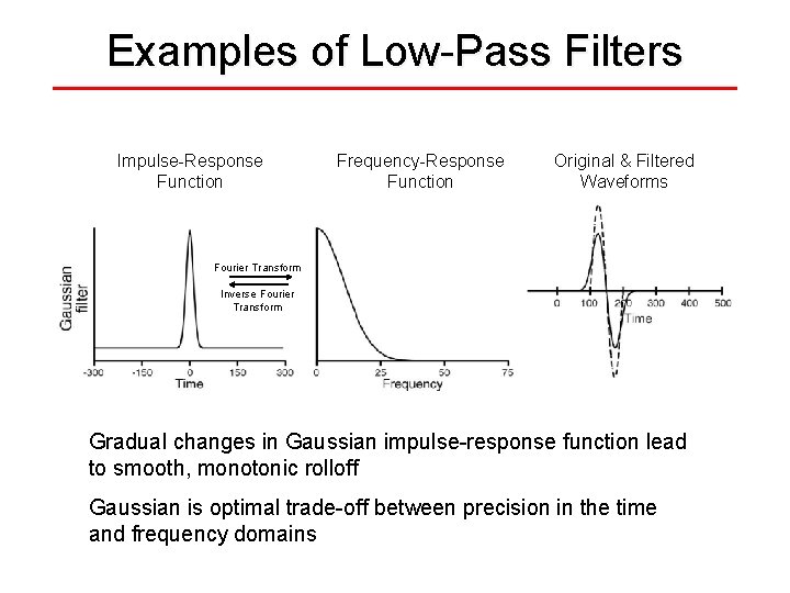
Examples of Low-Pass Filters Impulse-Response Function Frequency-Response Function Original & Filtered Waveforms Fourier Transform Inverse Fourier Transform Gradual changes in Gaussian impulse-response function lead to smooth, monotonic rolloff Gaussian is optimal trade-off between precision in the time and frequency domains
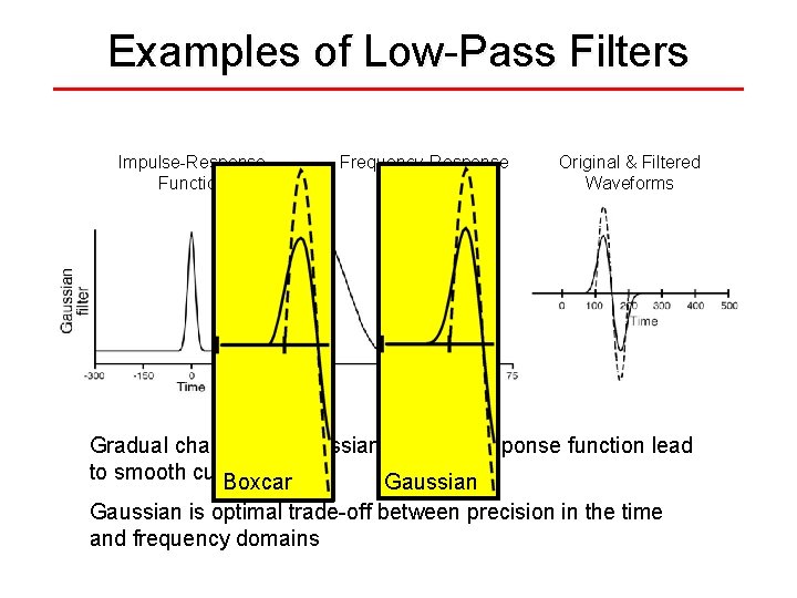
Examples of Low-Pass Filters Impulse-Response Function Frequency-Response Function Original & Filtered Waveforms Fourier Transform Inverse Fourier Transform Gradual changes in Gaussian impulse-response function lead to smooth cutoff Boxcar Gaussian is optimal trade-off between precision in the time and frequency domains
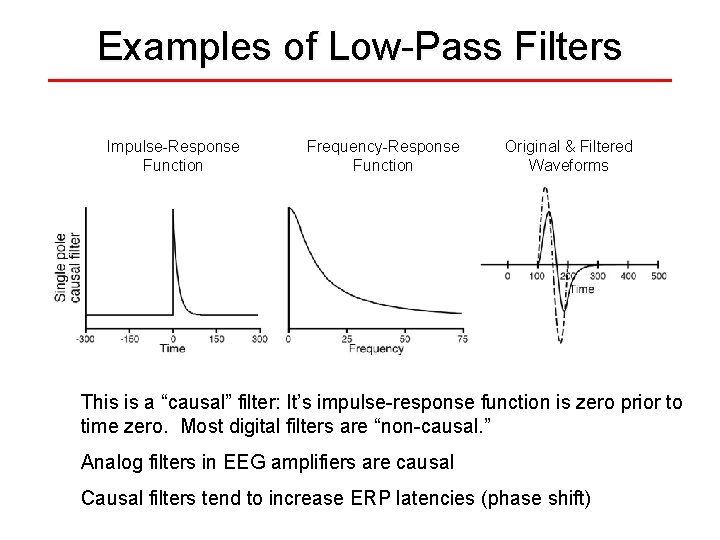
Examples of Low-Pass Filters Impulse-Response Function Frequency-Response Function Original & Filtered Waveforms This is a “causal” filter: It’s impulse-response function is zero prior to time zero. Most digital filters are “non-causal. ” Analog filters in EEG amplifiers are causal Causal filters tend to increase ERP latencies (phase shift)
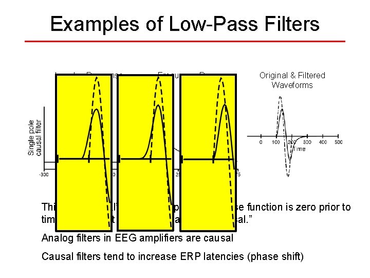
Examples of Low-Pass Filters Impulse-Response Function Frequency-Response Function Original & Filtered Waveforms This is a “causal” filter: It’s impulse-response function is zero prior to time zero. Most digital filters are “non-causal. ” Analog filters in EEG amplifiers are causal Causal filters tend to increase ERP latencies (phase shift)
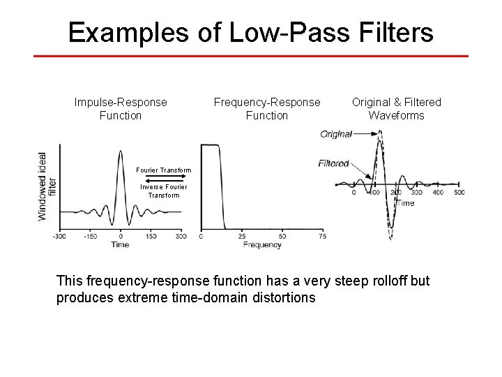
Examples of Low-Pass Filters Impulse-Response Function Frequency-Response Function Original & Filtered Waveforms Fourier Transform Inverse Fourier Transform This frequency-response function has a very steep rolloff but produces extreme time-domain distortions
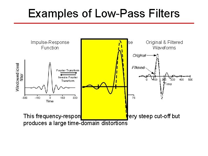
Examples of Low-Pass Filters Impulse-Response Function Frequency-Response Function Original & Filtered Waveforms Fourier Transform Inverse Fourier Transform This frequency-response function has a very steep cut-off but produces a large time-domain distortions
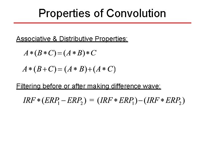
Properties of Convolution Associative & Distributive Properties: Filtering before or after making difference wave:
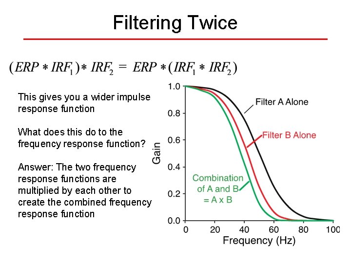
Filtering Twice This gives you a wider impulse response function What does this do to the frequency response function? Answer: The two frequency response functions are multiplied by each other to create the combined frequency response function
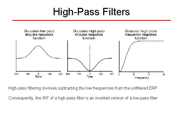
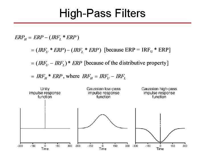
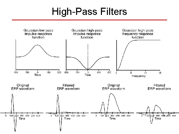
High-Pass Filters High-pass filtering involves subtracting the low frequencies from the unfiltered ERP Consequently, the IRF of a high-pass filter is an inverted version of a low-pass filter
High-Pass Filters
High-Pass Filters
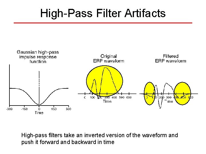
High-Pass Filter Artifacts High-pass filters take an inverted version of the waveform and push it forward and backward in time
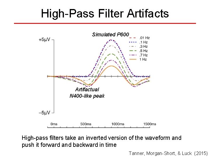
High-Pass Filter Artifacts Simulated P 600 Artifactual N 400 -like peak High-pass filters take an inverted version of the waveform and push it forward and backward in time Tanner, Morgan-Short, & Luck (2015)
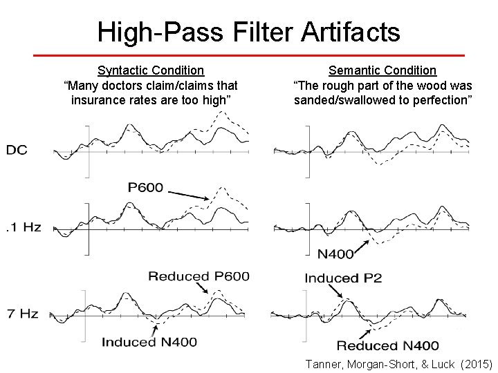
High-Pass Filter Artifacts Syntactic Condition “Many doctors claim/claims that insurance rates are too high” Semantic Condition “The rough part of the wood was sanded/swallowed to perfection” Tanner, Morgan-Short, & Luck (2015)
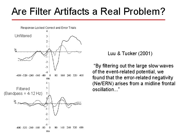
Are Filter Artifacts a Real Problem? Response-Locked Correct and Error Trials Unfiltered Luu & Tucker (2001) Filtered (Bandpass = 4 -12 Hz) “By filtering out the large slow waves of the event-related potential, we found that the error-related negativity (Ne/ERN) arises from a midline frontal oscillation. . . ”
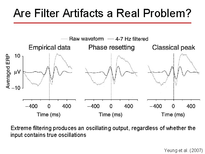
Are Filter Artifacts a Real Problem? Extreme filtering produces an oscillating output, regardless of whether the input contains true oscillations Yeung et al. (2007)
Recommendations- Online Filtering • Filter as little as possible online - You can’t “unfilter” filtered data • • • Low-pass filter at 1/3– 1/4 times the sampling rate Notch filters are usually OK if needed If you have 24+ bits - Record at DC - Record ~20 s of blank at beginning and end of each trial block • If you have <24 bits - High-pass filter cutoff between. 01 and. 1 Hz to avoid saturating the amplifier/ADC • • . 01 Hz for ideal conditions 0. 1 Hz for less-than-ideal conditions
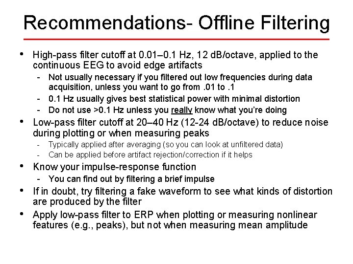
Recommendations- Offline Filtering • • • High-pass filter cutoff at 0. 01– 0. 1 Hz, 12 d. B/octave, applied to the continuous EEG to avoid edge artifacts - Not usually necessary if you filtered out low frequencies during data acquisition, unless you want to go from. 01 to. 1 - 0. 1 Hz usually gives best statistical power with minimal distortion - Do not use >0. 1 Hz unless you really know what you’re doing Low-pass filter cutoff at 20– 40 Hz (12 -24 d. B/octave) to reduce noise during plotting or when measuring peaks - Typically applied after averaging (so you can look at unfiltered data) - Can be applied before artifact rejection/correction if it helps Know your impulse-response function - You can find out by filtering a brief impulse If in doubt, try filtering a fake waveform to see what kinds of distortion are produced by the filter Apply low-pass filter to ERP when plotting or measuring nonlinear features (e. g. , peaks), but not when measuring mean amplitude
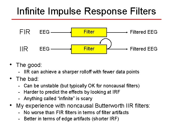
Infinite Impulse Response Filters • • • FIR EEG Filtered EEG IIR EEG Filtered EEG The good: - IIR can achieve a sharper rolloff with fewer data points The bad: - Can be unstable (but typically OK for noncausal filters) Harder to predict the effects by looking at IRF Anything called “infinite” is scary My experience with noncausal Butterworth IIR filters: - No worse than FIR filters in terms of filter artifacts - Better in terms of edge artifacts (shorter IRF)
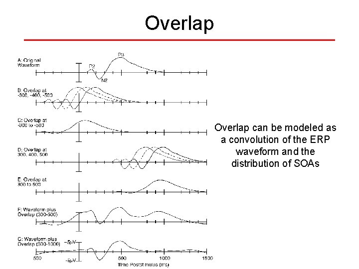
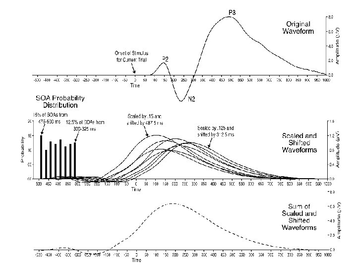
Overlap can be modeled as a convolution of the ERP waveform and the distribution of SOAs
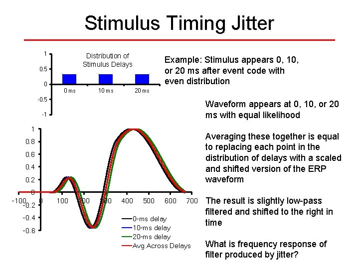
Stimulus Timing Jitter 1 Distribution of Stimulus Delays 0. 5 Example: Stimulus appears 0, 10, or 20 ms after event code with even distribution 0 0 ms 10 ms 20 ms -0. 5 Waveform appears at 0, 10, or 20 ms with equal likelihood -1 1 Averaging these together is equal to replacing each point in the distribution of delays with a scaled and shifted version of the ERP waveform 0. 8 0. 6 0. 4 0. 2 0 -100 0 -0. 2 -0. 4 -0. 6 100 200 300 400 500 600 700 0 -ms delay 10 -ms delay 20 -ms delay Avg Across Delays The result is slightly low-pass filtered and shifted to the right in time What is frequency response of filter produced by jitter?
- Slides: 57