Theory of electric networks The twopoint resistance and

Theory of electric networks: The two-point resistance and impedance F. Y. Wu Northeastern University Boston, Massachusetts USA

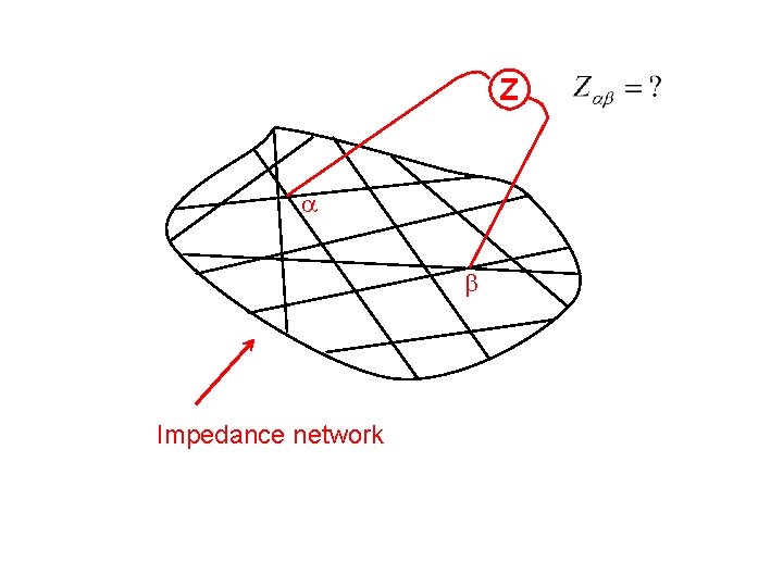
Z a b Impedance network

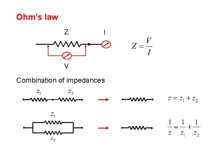
Ohm’s law Z I V Combination of impedances

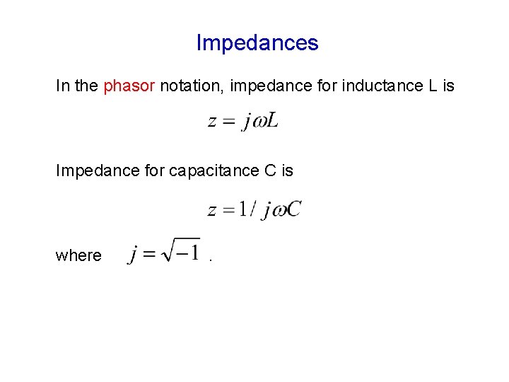
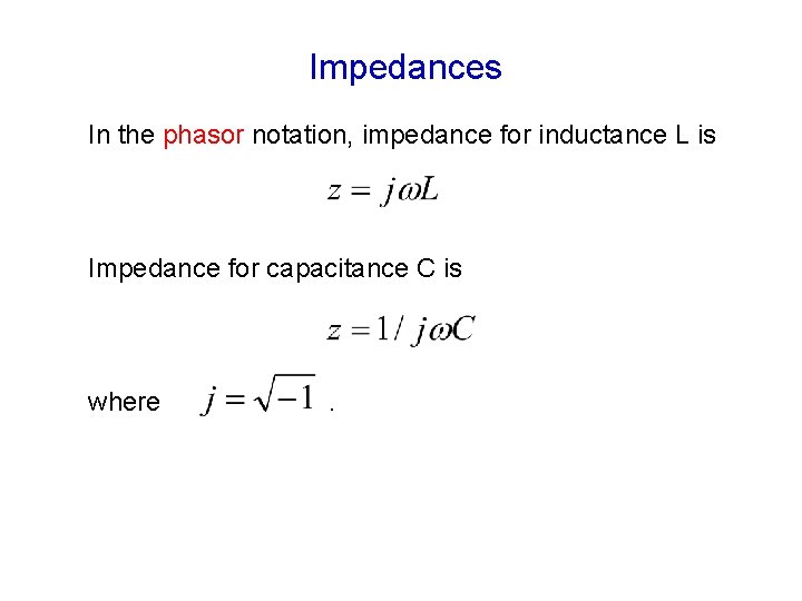
Impedances In the phasor notation, impedance for inductance L is Impedance for capacitance C is where .

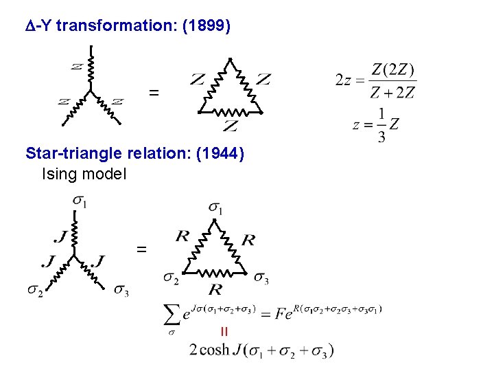
D-Y transformation: (1899) = Star-triangle relation: (1944) Ising model = =

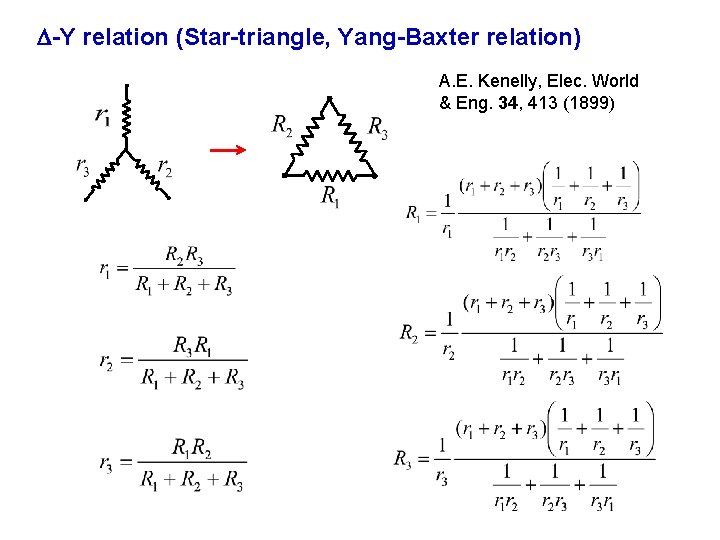
D-Y relation (Star-triangle, Yang-Baxter relation) A. E. Kenelly, Elec. World & Eng. 34, 413 (1899)

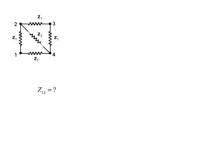
z 1 3 2 z 1 1 z 2 z 1 4

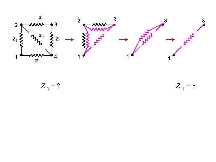
z 1 3 2 z 1 1 z 2 z 1 2 3 3 3 z 1 4 1 1 1

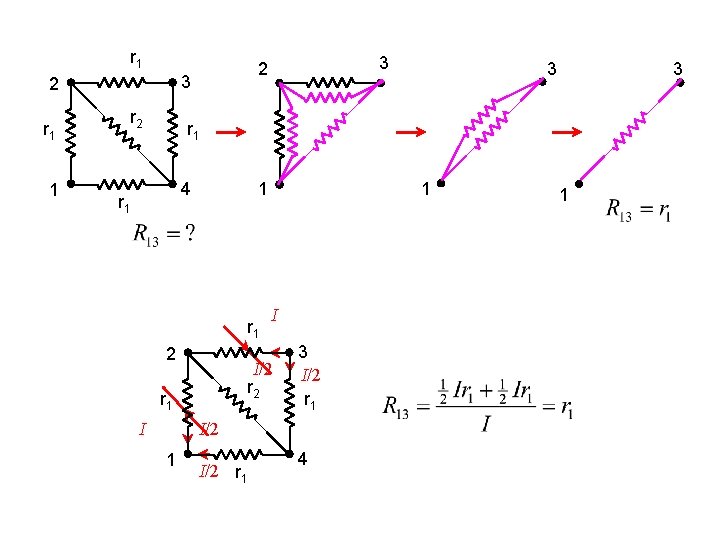
r 1 3 2 r 1 1 r 2 3 3 r 1 4 r 1 1 r 1 2 I I/2 r 1 I 1 3 I/2 r 1 4 1

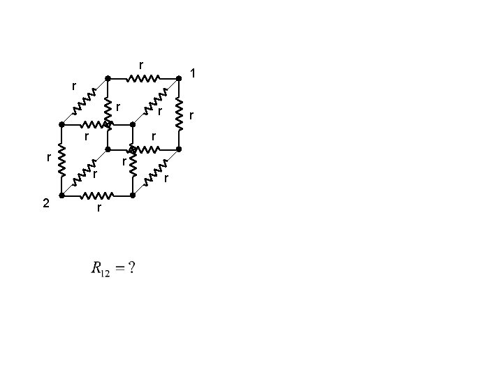
r 1 r r r r 2 r r r

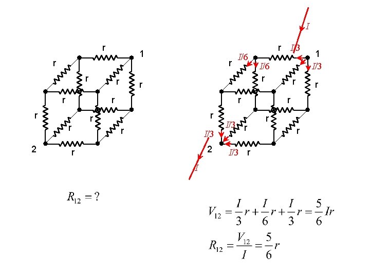
I r 1 r r r r r I/3 2 r I I/3 r I/3 I/6 r r 2 r I/6 r r 1 I/3 r r

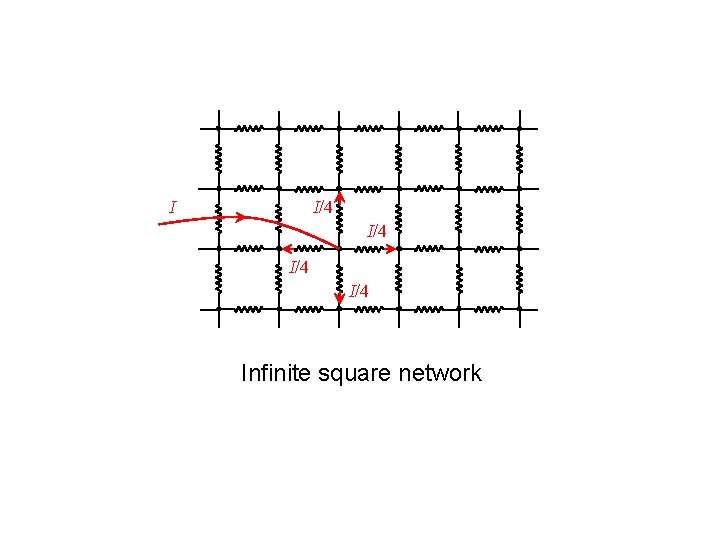
I I/4 I/4 Infinite square network

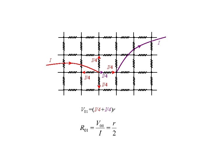
I I I/4 I/4 I/4 V 01=(I/4+I/4)r

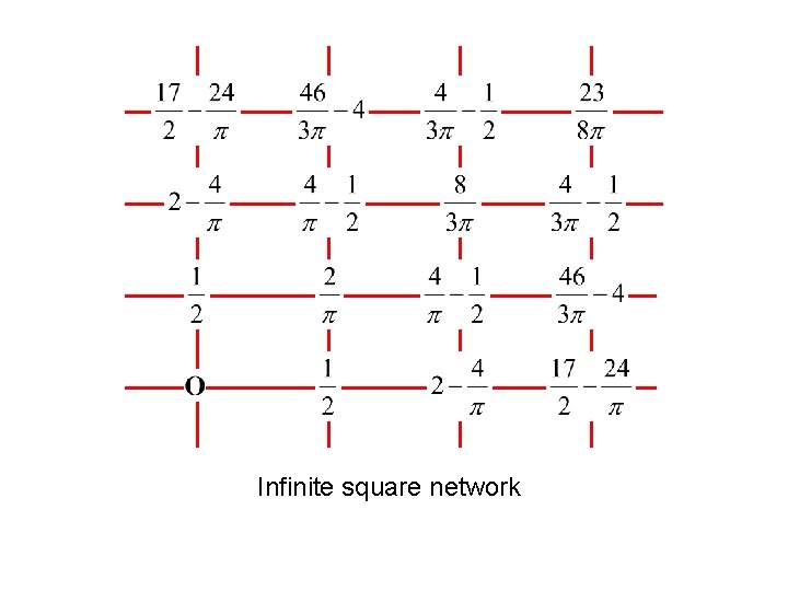
Infinite square network

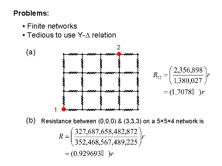
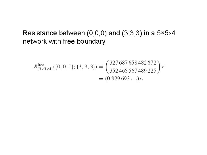
Problems: • Finite networks • Tedious to use Y-D relation 2 (a) 1 (b) Resistance between (0, 0, 0) & (3, 3, 3) on a 5× 5× 4 network is

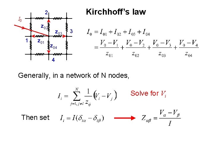
Kirchhoff’s law 2 I 0 z 02 1 z 03 3 z 04 4 Generally, in a network of N nodes, Solve for Vi Then set

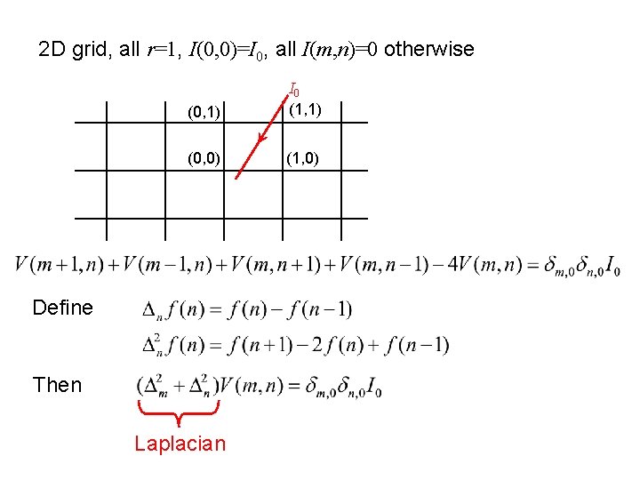
2 D grid, all r=1, I(0, 0)=I 0, all I(m, n)=0 otherwise (0, 1) I 0 (1, 1) (0, 0) (1, 0) Define Then Laplacian

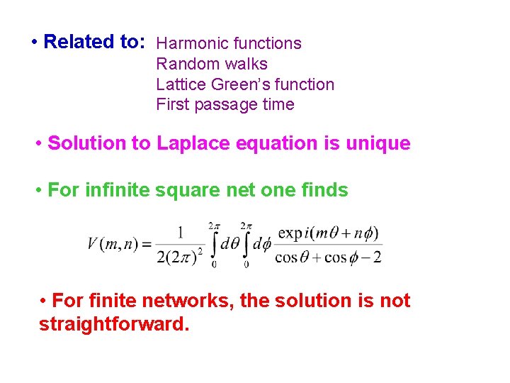
• Related to: Harmonic functions Random walks Lattice Green’s function First passage time • Solution to Laplace equation is unique • For infinite square net one finds • For finite networks, the solution is not straightforward.

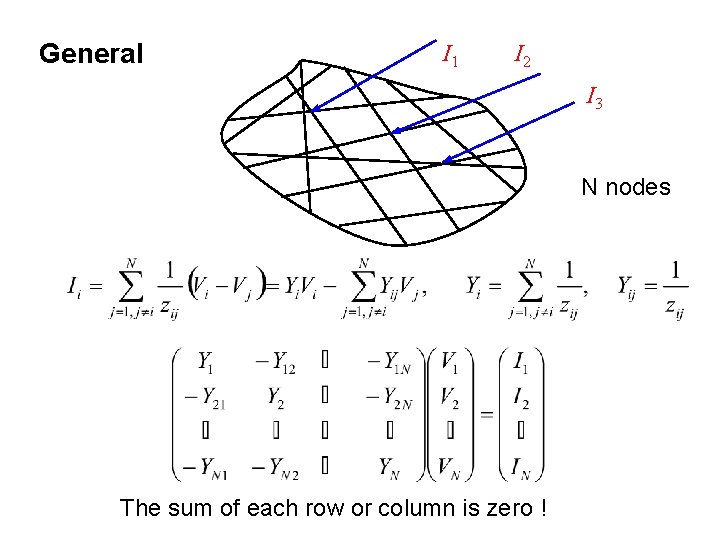
General I 1 I 2 I 3 N nodes The sum of each row or column is zero !

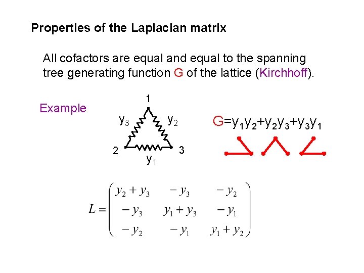
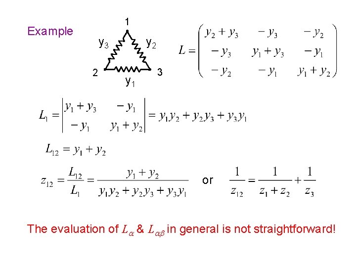
Properties of the Laplacian matrix All cofactors are equal and equal to the spanning tree generating function G of the lattice (Kirchhoff). 1 Example y 3 2 y 1 G=y 1 y 2+y 2 y 3+y 3 y 1 3

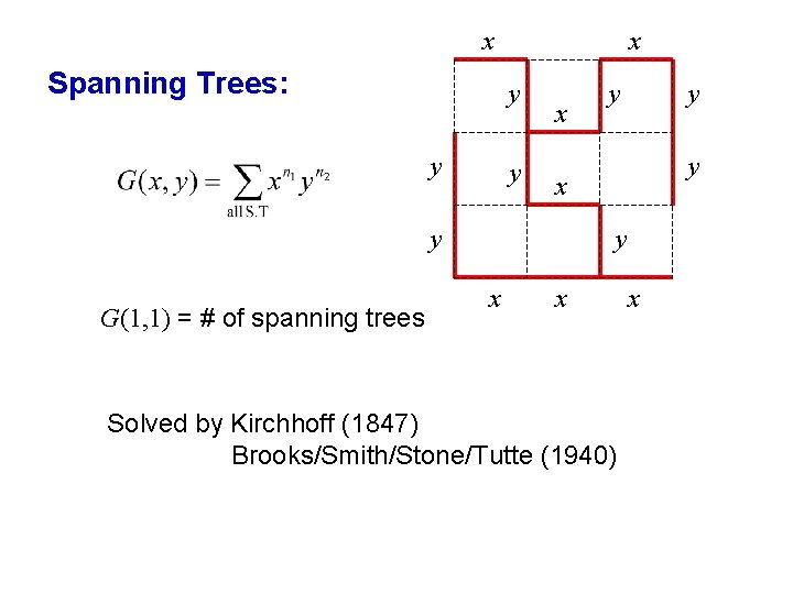
x Spanning Trees: x y y y x y G(1, 1) = # of spanning trees y y x x Solved by Kirchhoff (1847) Brooks/Smith/Stone/Tutte (1940) x

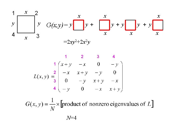
1 x 2 y y 4 3 x x x y+ G(x, y)= y x y+y x x =2 xy 2+2 x 2 y 1 1 2 3 4 N=4 2 3 y + y 4 x

General I 1 I 2 I 3 N nodes The sum of each row or column is zero !

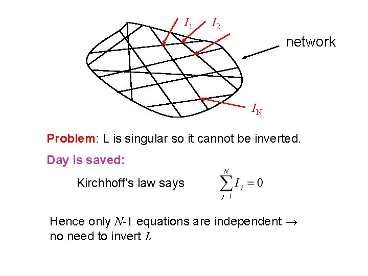
I 1 I 2 network IN Problem: L is singular so it cannot be inverted. Day is saved: Kirchhoff’s law says Hence only N-1 equations are independent → no need to invert L

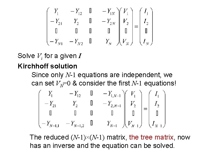
Solve Vi for a given I Kirchhoff solution Since only N-1 equations are independent, we can set VN=0 & consider the first N-1 equations! The reduced (N-1)×(N-1) matrix, the tree matrix, now has an inverse and the equation can be solved.

1 Example y 3 2 y 1 3 or The evaluation of La & Lab in general is not straightforward!

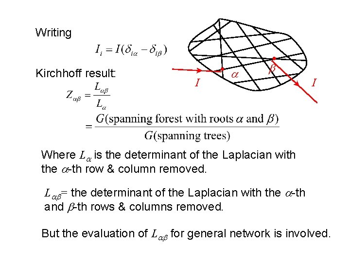
Writing Kirchhoff result: I a b I Where La is the determinant of the Laplacian with the a-th row & column removed. Lab= the determinant of the Laplacian with the a-th and b-th rows & columns removed. But the evaluation of Lab for general network is involved.

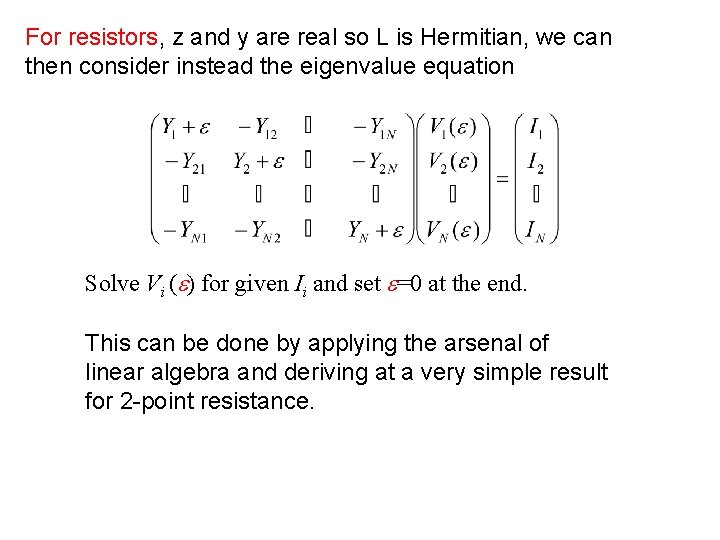
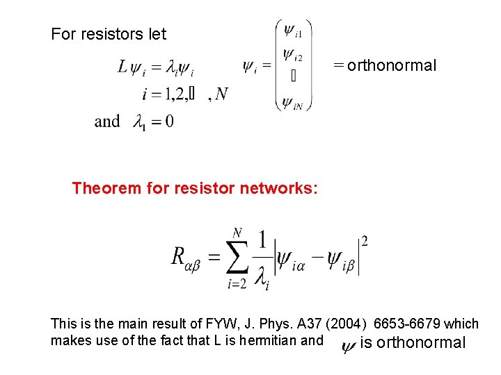
For resistors, z and y are real so L is Hermitian, we can then consider instead the eigenvalue equation Solve Vi (e) for given Ii and set e=0 at the end. This can be done by applying the arsenal of linear algebra and deriving at a very simple result for 2 -point resistance.

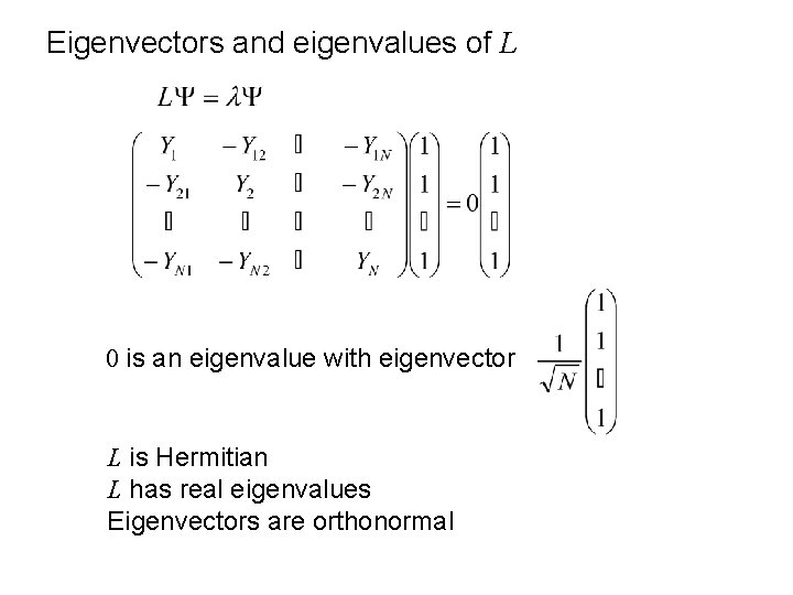
Eigenvectors and eigenvalues of L 0 is an eigenvalue with eigenvector L is Hermitian L has real eigenvalues Eigenvectors are orthonormal

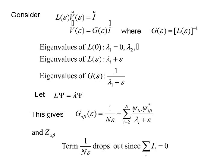
Consider where Let This gives

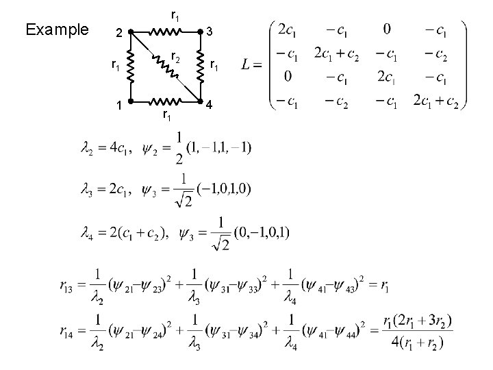
Example r 1 3 2 r 1 1 r 2 r 1 4

For resistors let = orthonormal Theorem for resistor networks: This is the main result of FYW, J. Phys. A 37 (2004) 6653 -6679 which makes use of the fact that L is hermitian and is orthonormal

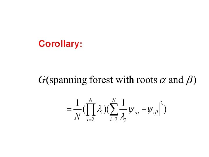
Corollary:

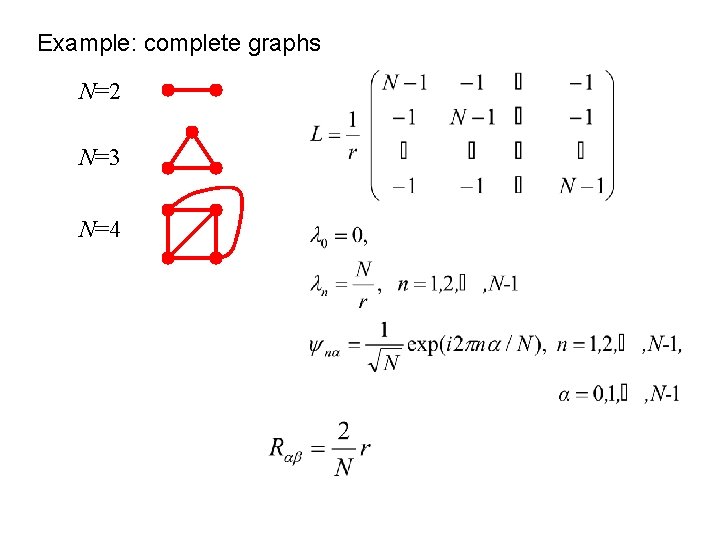
Example: complete graphs N=2 N=3 N=4

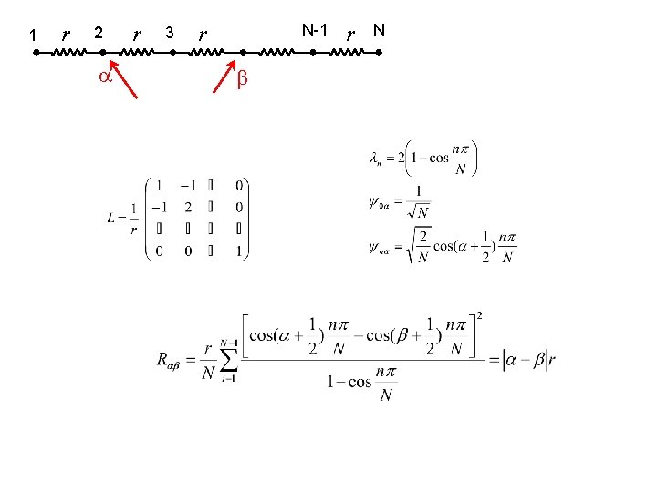
1 r 2 a r 3 N-1 r b r N

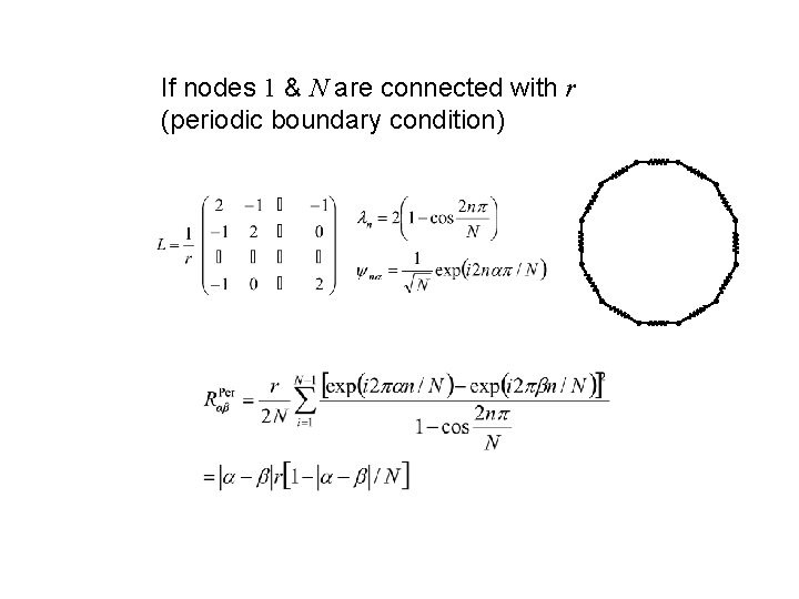
If nodes 1 & N are connected with r (periodic boundary condition)

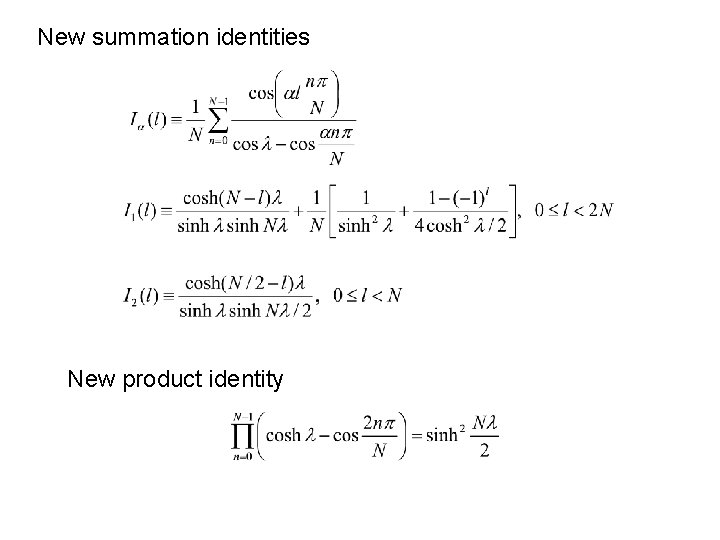
New summation identities New product identity

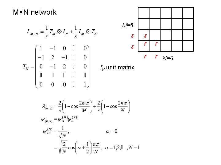
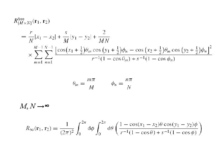
M×N network M=5 s s s r r N=6 IN unit matrix

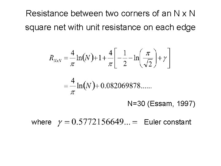
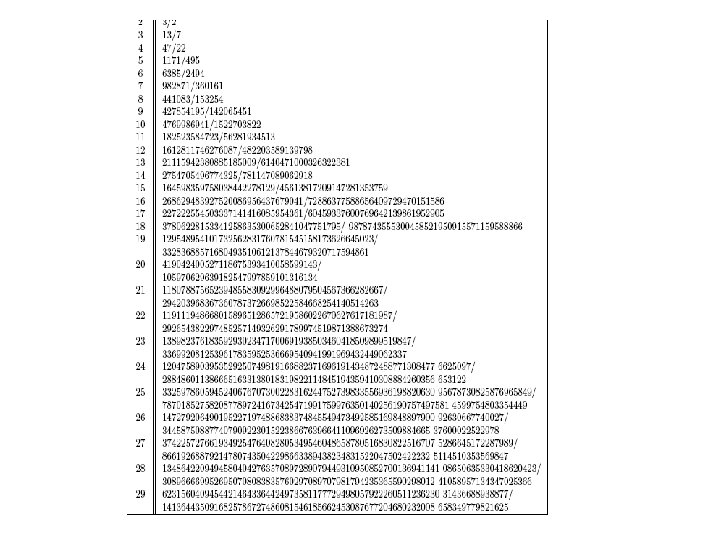
Resistance between two corners of an N x N square net with unit resistance on each edge N=30 (Essam, 1997) where Euler constant

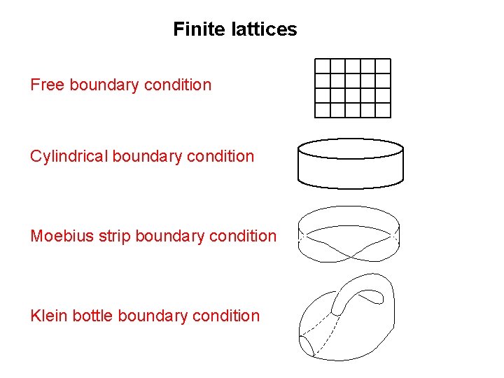
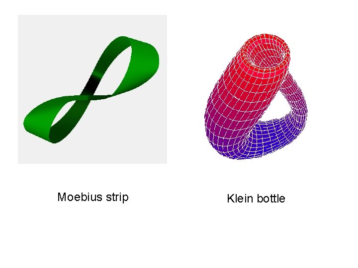
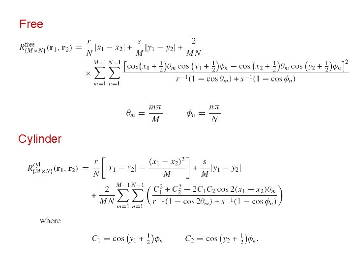
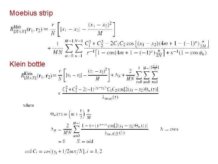
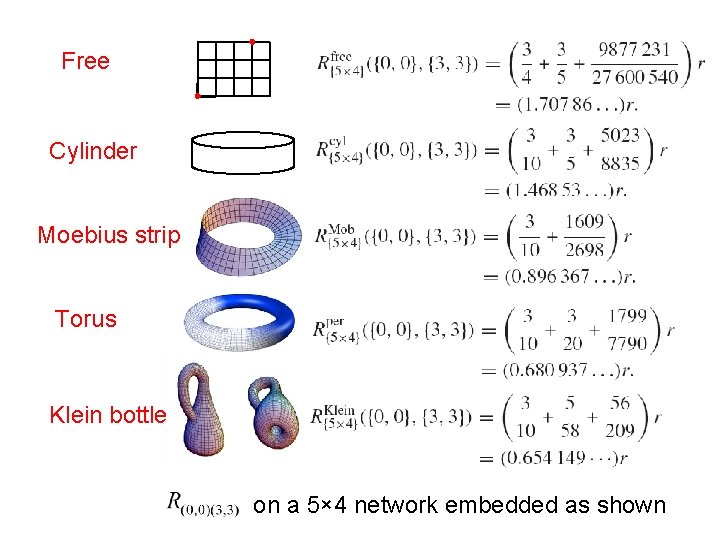
Finite lattices Free boundary condition Cylindrical boundary condition Moebius strip boundary condition Klein bottle boundary condition

Moebius strip Klein bottle

Free Cylinder

Moebius strip Klein bottle

Free Cylinder Moebius strip Torus Klein bottle on a 5× 4 network embedded as shown

Resistance between (0, 0, 0) and (3, 3, 3) in a 5× 5× 4 network with free boundary

Impedances In the phasor notation, impedance for inductance L is Impedance for capacitance C is where .

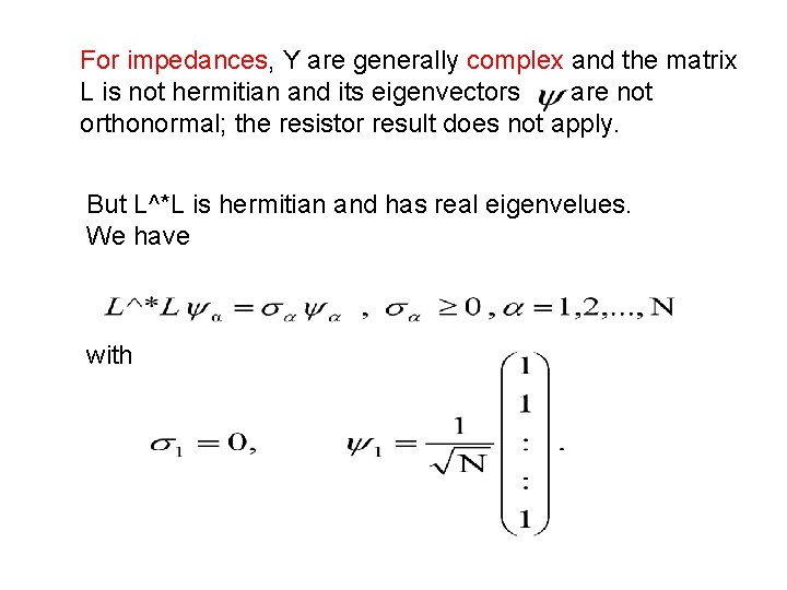
For impedances, Y are generally complex and the matrix L is not hermitian and its eigenvectors are not orthonormal; the resistor result does not apply. But L^*L is hermitian and has real eigenvelues. We have with

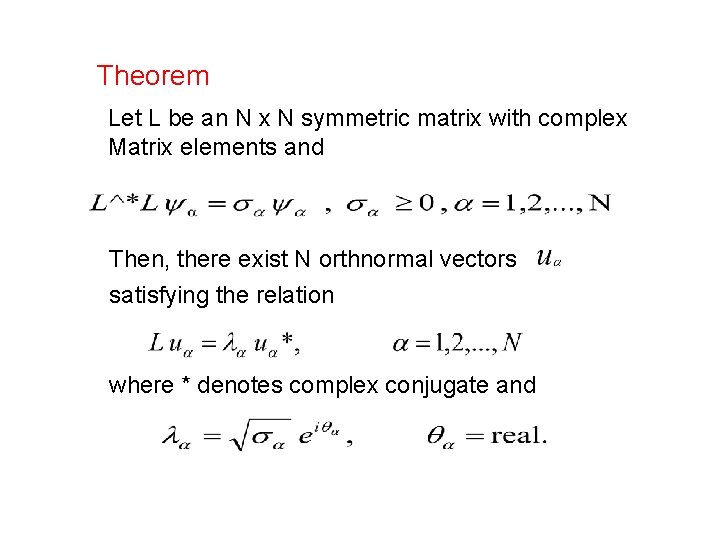
Theorem Let L be an N x N symmetric matrix with complex Matrix elements and Then, there exist N orthnormal vectors satisfying the relation where * denotes complex conjugate and

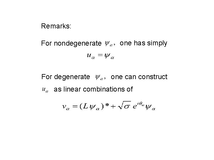
Remarks: For nondegenerate For degenerate one has simply one can construct as linear combinations of

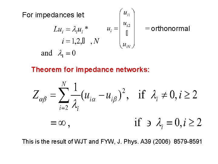
For impedances let = orthonormal Theorem for impedance networks: This is the result of WJT and FYW, J. Phys. A 39 (2006) 8579 -8591

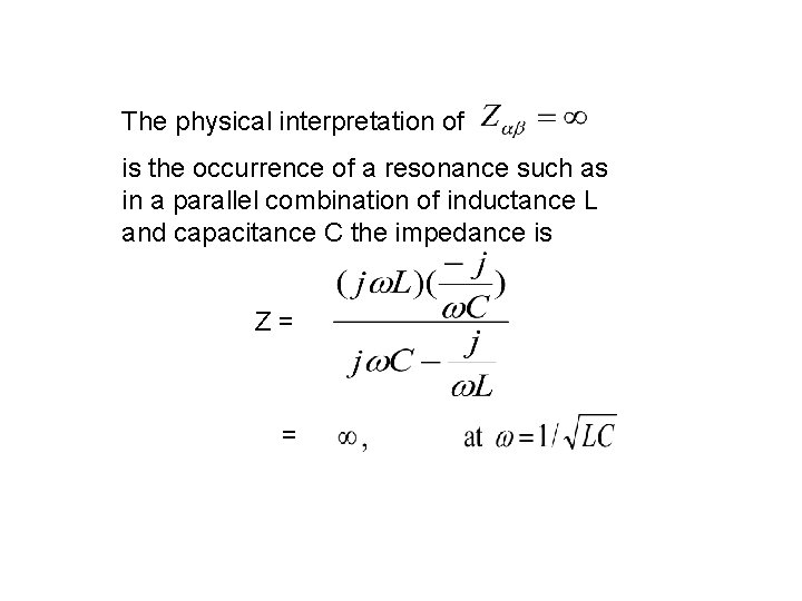
The physical interpretation of is the occurrence of a resonance such as in a parallel combination of inductance L and capacitance C the impedance is Z= =

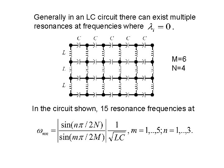
Generally in an LC circuit there can exist multiple resonances at frequencies where M=6 N=4 In the circuit shown, 15 resonance frequencies at

Summary • An elegant formulation of computing twopoint impedances in a network, a problem lingering since the Kirchhoff time. • Prediction of the occurrence of multiresonances in a network consisting of reactances L and C, a prediction which may have practical relevance.

FYW, J. Phys. A 37 (2004) 6653 -6673 W-J Tzeng and FYW, J. Phys. A 39 (2006), 8579 -8591