The theory of demand The theory of demand

The theory of demand

The theory of demand • • Optimal choice and demand Change in the price of a good: substitution effect and income effect Change in the price of a good: the consumption of the consumer surplus Market demand Network externalities The choice of labor and liesure Consumer price indices

How and What ? How a consumer’s demand for a good depends on the prices of all goods and on income? What happens to the consumer’s choice of food when the price of food changes while the price of clothing and the amount of income remain constant?

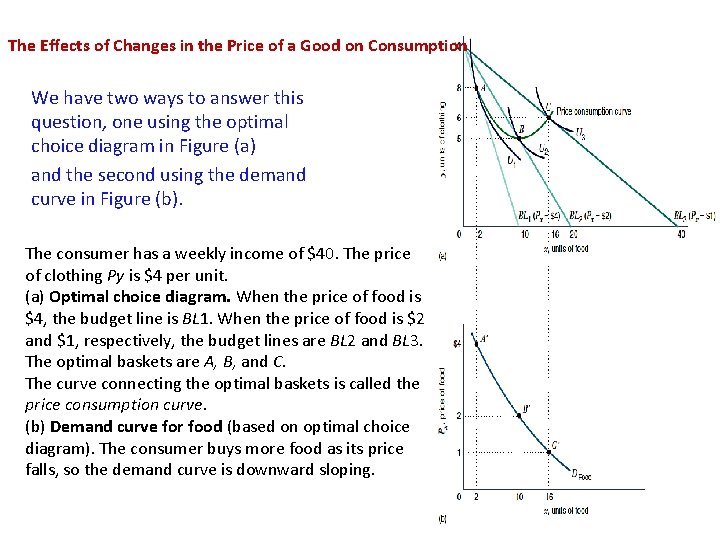
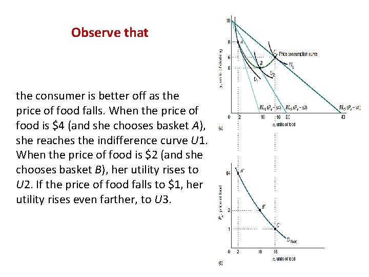
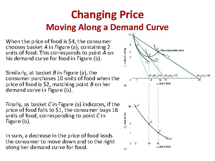
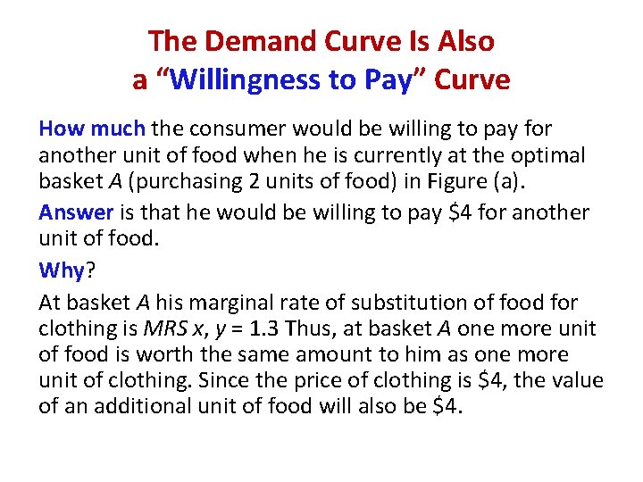
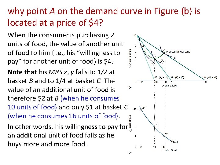
The Effects of Changes in the Price of a Good on Consumption We have two ways to answer this question, one using the optimal choice diagram in Figure (a) and the second using the demand curve in Figure (b). The consumer has a weekly income of $40. The price of clothing Py is $4 per unit. (a) Optimal choice diagram. When the price of food is $4, the budget line is BL 1. When the price of food is $2 and $1, respectively, the budget lines are BL 2 and BL 3. The optimal baskets are A, B, and C. The curve connecting the optimal baskets is called the price consumption curve. (b) Demand curve for food (based on optimal choice diagram). The consumer buys more food as its price falls, so the demand curve is downward sloping.

Observe that the consumer is better off as the price of food falls. When the price of food is $4 (and she chooses basket A), she reaches the indifference curve U 1. When the price of food is $2 (and she chooses basket B), her utility rises to U 2. If the price of food falls to $1, her utility rises even farther, to U 3.

Changing Price Moving Along a Demand Curve When the price of food is $4, the consumer chooses basket A in Figure (a), containing 2 units of food. This corresponds to point A on his demand curve for food in Figure (b). Similarly, at basket B in Figure (a), the consumer purchases 10 units of food when the price of food is $2, matching point B on her demand curve in Figure (b). Finally, as basket C in Figure (a) indicates, if the price of food falls to $1, the consumer buys 16 units of food, corresponding to point C in Figure (b). In sum, a decrease in the price of food leads the consumer to move down and to the right along her demand curve for food.

The Demand Curve Is Also a “Willingness to Pay” Curve How much the consumer would be willing to pay for another unit of food when he is currently at the optimal basket A (purchasing 2 units of food) in Figure (a). Answer is that he would be willing to pay $4 for another unit of food. Why? At basket A his marginal rate of substitution of food for clothing is MRS x, y = 1. 3 Thus, at basket A one more unit of food is worth the same amount to him as one more unit of clothing. Since the price of clothing is $4, the value of an additional unit of food will also be $4.

why point A on the demand curve in Figure (b) is located at a price of $4? When the consumer is purchasing 2 units of food, the value of another unit of food to him (i. e. , his “willingness to pay” for another unit of food) is $4. Note that his MRS x, y falls to 1/2 at basket B and to 1/4 at basket C. The value of an additional unit of food is therefore $2 at B (when he consumes 10 units of food) and only $1 at basket C (when he consumes 16 units of food). In other words, his willingness to pay for an additional unit of food falls as he buys more and more food.

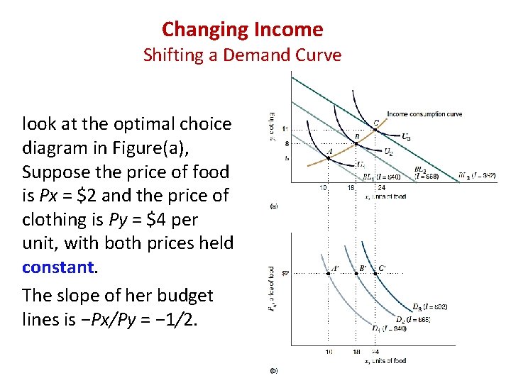
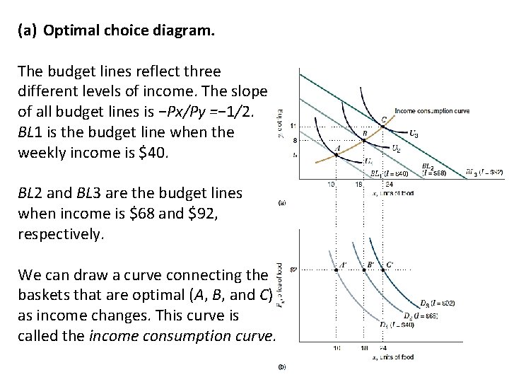
Changing Income Shifting a Demand Curve look at the optimal choice diagram in Figure(a), Suppose the price of food is Px = $2 and the price of clothing is Py = $4 per unit, with both prices held constant. The slope of her budget lines is −Px/Py = − 1/2.

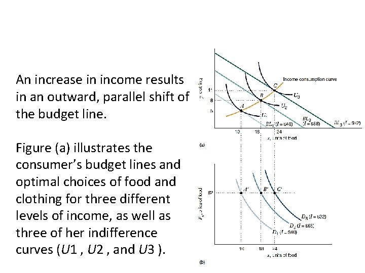
An increase in income results in an outward, parallel shift of the budget line. Figure (a) illustrates the consumer’s budget lines and optimal choices of food and clothing for three different levels of income, as well as three of her indifference curves (U 1 , U 2 , and U 3 ).

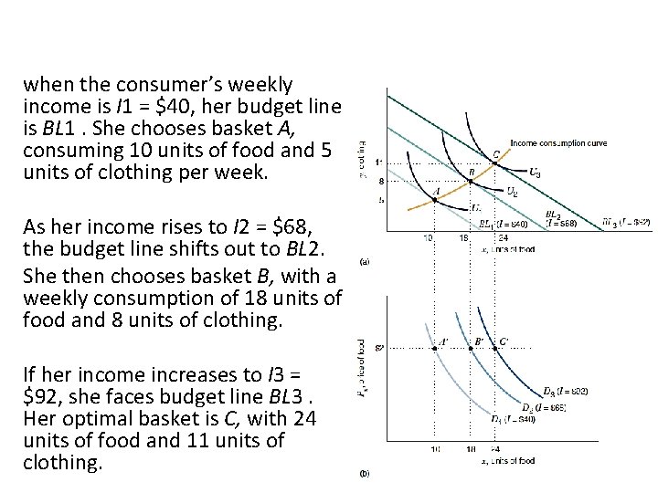
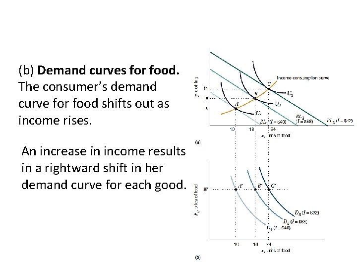
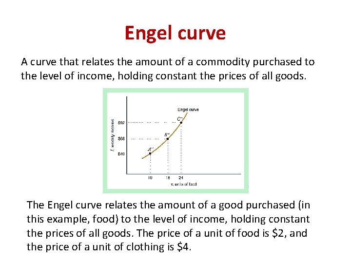
when the consumer’s weekly income is I 1 = $40, her budget line is BL 1. She chooses basket A, consuming 10 units of food and 5 units of clothing per week. As her income rises to I 2 = $68, the budget line shifts out to BL 2. She then chooses basket B, with a weekly consumption of 18 units of food and 8 units of clothing. If her income increases to I 3 = $92, she faces budget line BL 3. Her optimal basket is C, with 24 units of food and 11 units of clothing.

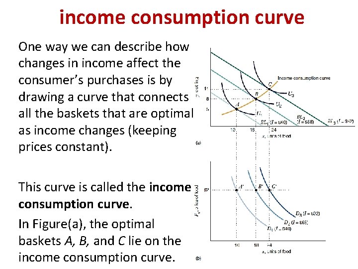
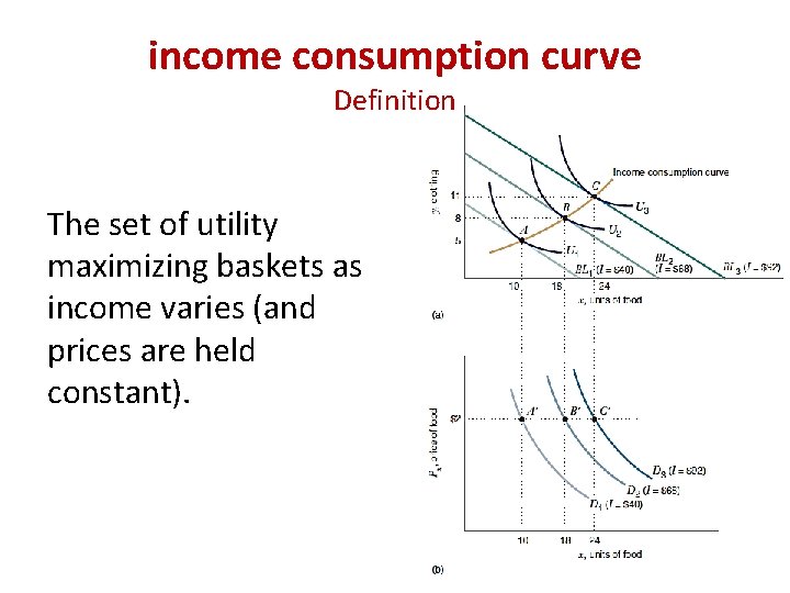
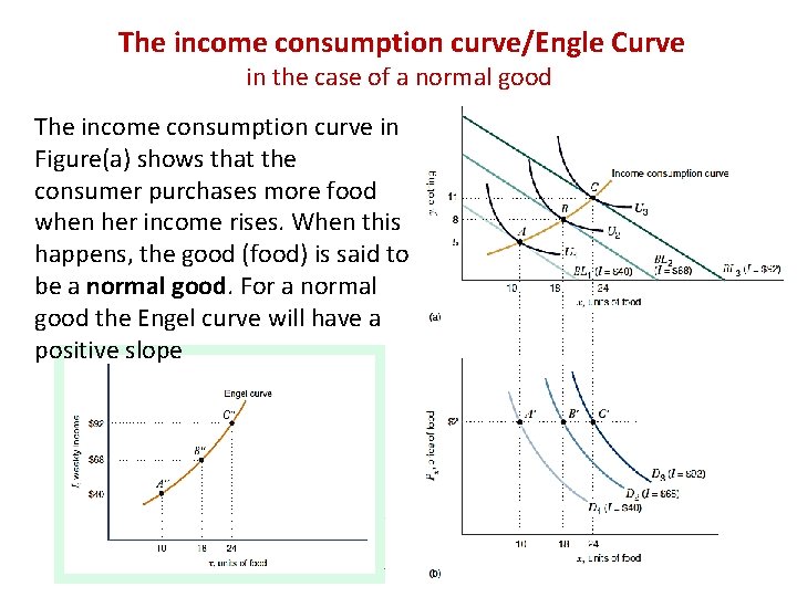
income consumption curve One way we can describe how changes in income affect the consumer’s purchases is by drawing a curve that connects all the baskets that are optimal as income changes (keeping prices constant). This curve is called the income consumption curve. In Figure(a), the optimal baskets A, B, and C lie on the income consumption curve.

The consumer buys food at Px $2 per unit and clothing at Py $4 per unit. Both prices are held constant as income varies.

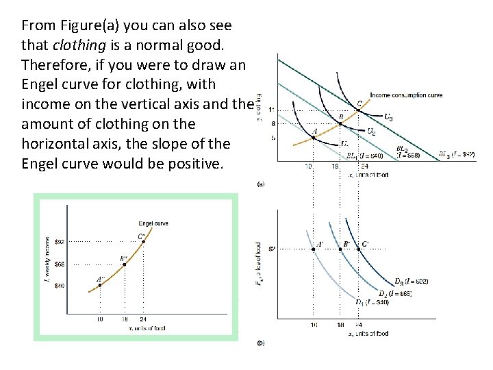
(a) Optimal choice diagram. The budget lines reflect three different levels of income. The slope of all budget lines is −Px/Py =− 1/2. BL 1 is the budget line when the weekly income is $40. BL 2 and BL 3 are the budget lines when income is $68 and $92, respectively. We can draw a curve connecting the baskets that are optimal (A, B, and C) as income changes. This curve is called the income consumption curve.

(b) Demand curves for food. The consumer’s demand curve for food shifts out as income rises. An increase in income results in a rightward shift in her demand curve for each good.

income consumption curve Definition The set of utility maximizing baskets as income varies (and prices are held constant).

Engel curve A curve that relates the amount of a commodity purchased to the level of income, holding constant the prices of all goods. The Engel curve relates the amount of a good purchased (in this example, food) to the level of income, holding constant the prices of all goods. The price of a unit of food is $2, and the price of a unit of clothing is $4.

The income consumption curve/Engle Curve in the case of a normal good The income consumption curve in Figure(a) shows that the consumer purchases more food when her income rises. When this happens, the good (food) is said to be a normal good. For a normal good the Engel curve will have a positive slope

From Figure(a) you can also see that clothing is a normal good. Therefore, if you were to draw an Engel curve for clothing, with income on the vertical axis and the amount of clothing on the horizontal axis, the slope of the Engel curve would be positive.

Consumers don’t always purchase more of every good as income rises. If a consumer wants to buy less of a good when income rises, that good is termed an … inferior good.

• normal …………. . …. good A good that a consumer purchases more of as income rises. • inferior good A good that a consumer …………………. purchases less of as income rises.

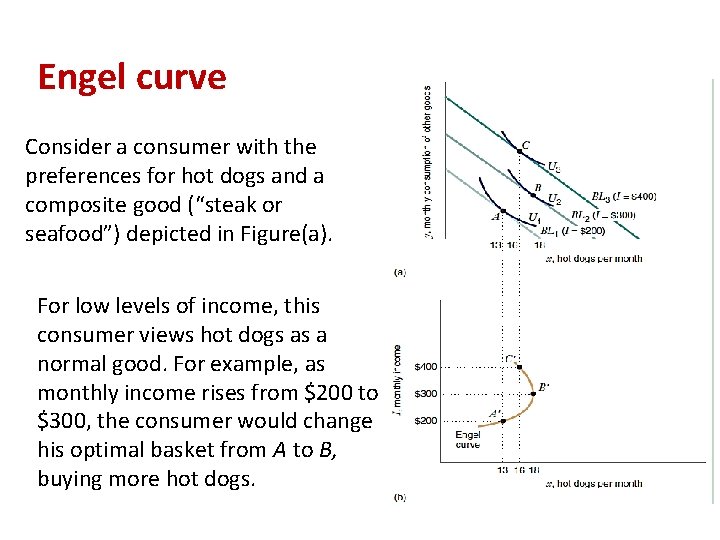
Engel curve Consider a consumer with the preferences for hot dogs and a composite good (“steak or seafood”) depicted in Figure(a). For low levels of income, this consumer views hot dogs as a normal good. For example, as monthly income rises from $200 to $300, the consumer would change his optimal basket from A to B, buying more hot dogs.

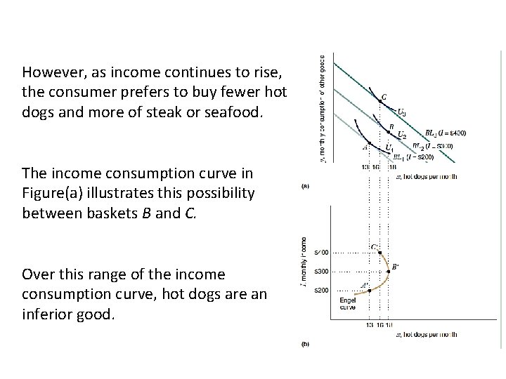
However, as income continues to rise, the consumer prefers to buy fewer hot dogs and more of steak or seafood. The income consumption curve in Figure(a) illustrates this possibility between baskets B and C. Over this range of the income consumption curve, hot dogs are an inferior good.

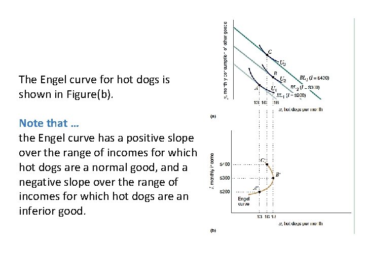
The Engel curve for hot dogs is shown in Figure(b). Note that … the Engel curve has a positive slope over the range of incomes for which hot dogs are a normal good, and a negative slope over the range of incomes for which hot dogs are an inferior good.

Problem A consumer likes to attend rock concerts and consume other goods. Suppose x measures the number of rock concerts he attends each year, and I denotes his annual income. Show that the following statement is true: If he views rock concerts as a normal good, Proof that his income elasticity of demand for rock concerts must be positive.

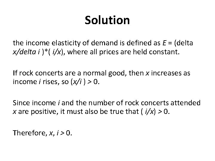
Solution the income elasticity of demand is defined as E = (delta x/delta i )*( i/x), where all prices are held constant. If rock concerts are a normal good, then x increases as income i rises, so (x/i ) > 0. Since income i and the number of rock concerts attended x are positive, it must also be true that ( i/x) > 0. Therefore, x, i > 0.

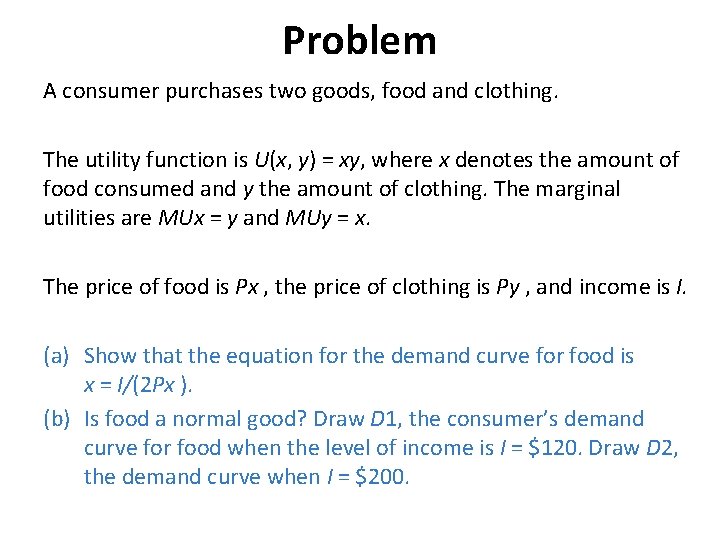
Problem A consumer purchases two goods, food and clothing. The utility function is U(x, y) = xy, where x denotes the amount of food consumed and y the amount of clothing. The marginal utilities are MUx = y and MUy = x. The price of food is Px , the price of clothing is Py , and income is I. (a) Show that the equation for the demand curve for food is x = I/(2 Px ). (b) Is food a normal good? Draw D 1, the consumer’s demand curve for food when the level of income is I = $120. Draw D 2, the demand curve when I = $200.

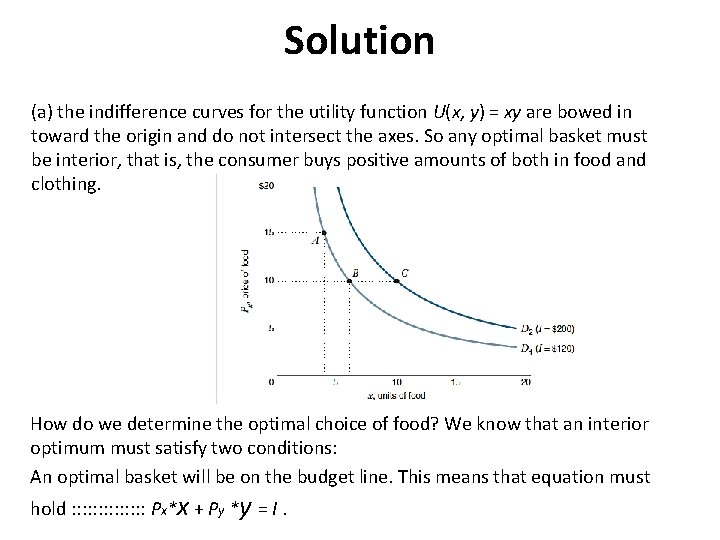
Solution (a) the indifference curves for the utility function U(x, y) = xy are bowed in toward the origin and do not intersect the axes. So any optimal basket must be interior, that is, the consumer buys positive amounts of both in food and clothing. How do we determine the optimal choice of food? We know that an interior optimum must satisfy two conditions: An optimal basket will be on the budget line. This means that equation must hold : : : : Px*x + Py *y = I.

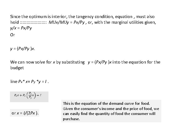
Since the optimum is interior, the tangency condition, equation , must also hold : : : : : : MUx/MUy = Px/Py , or, with the marginal utilities given, y/x = Px/Py Or y = (Px/Py )x. We can now solve for x by substituting y = (Px/Py )x into the equation for the budget line Px* x+ Py *y = I. or x = I/(2 Px ). This is the equation of the demand curve for food. Given the consumer’s income and the price of food, we can easily find the quantity of food the consumer will purchase.

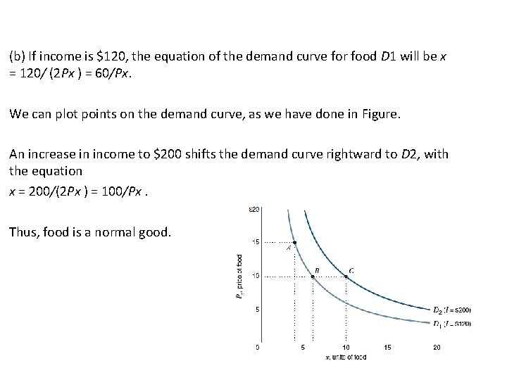
(b) If income is $120, the equation of the demand curve for food D 1 will be x = 120/ (2 Px ) = 60/Px. We can plot points on the demand curve, as we have done in Figure. An increase in income to $200 shifts the demand curve rightward to D 2, with the equation x = 200/(2 Px ) = 100/Px. Thus, food is a normal good.

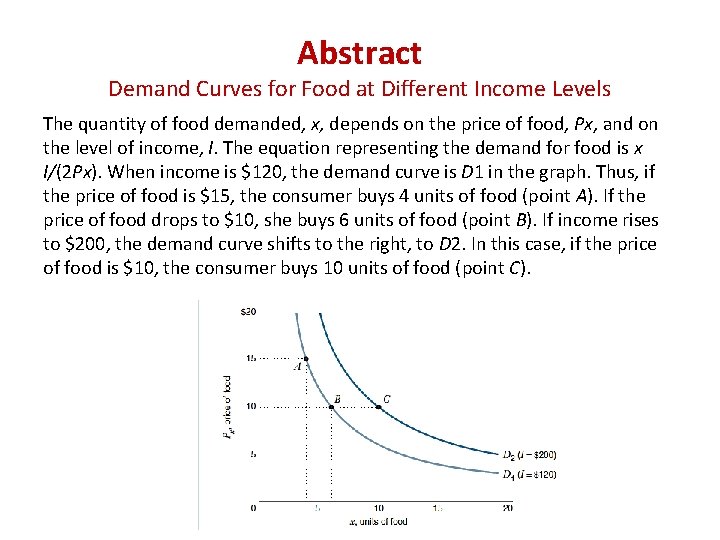
Abstract Demand Curves for Food at Different Income Levels The quantity of food demanded, x, depends on the price of food, Px, and on the level of income, I. The equation representing the demand for food is x I/(2 Px). When income is $120, the demand curve is D 1 in the graph. Thus, if the price of food is $15, the consumer buys 4 units of food (point A). If the price of food drops to $10, she buys 6 units of food (point B). If income rises to $200, the demand curve shifts to the right, to D 2. In this case, if the price of food is $10, the consumer buys 10 units of food (point C).

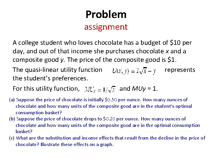
Problem assignment A college student who loves chocolate has a budget of $10 per day, and out of that income she purchases chocolate x and a composite good y. The price of the composite good is $1. The quasi-linear utility function represents the student’s preferences. For this utility function, and MUy = 1. (a) Suppose the price of chocolate is initially $0. 50 per ounce. How many ounces of chocolate and how many units of the composite good are in the student’s optimal consumption basket? (b) Suppose the price of chocolate drops to $0. 20 per ounce. How many ounces of chocolate and how many units of the composite good are in the optimal consumption basket? (c) What are the substitution and income effects that result from the decline in the price of chocolate? Illustrate these effects on a graph.

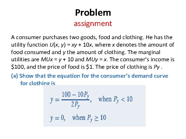
Problem assignment A consumer purchases two goods, food and clothing. He has the utility function U(x, y) = xy + 10 x, where x denotes the amount of food consumed and y the amount of clothing. The marginal utilities are MUx = y + 10 and MUy = x. The consumer’s income is $100, and the price of food is $1. The price of clothing is Py. (a) Show that the equation for the consumer’s demand curve for clothing is

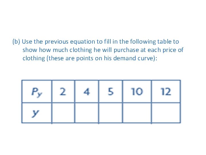
(b) Use the previous equation to fill in the following table to show much clothing he will purchase at each price of clothing (these are points on his demand curve):

The substitution effect normal good Suppose that a consumer buys two goods, food and clothing, that both goods have a positive marginal utility, and that the price of food decreases. The substitution effect is the amount of additional food the consumer would buy to achieve the same level of utility.

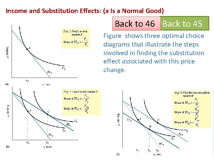
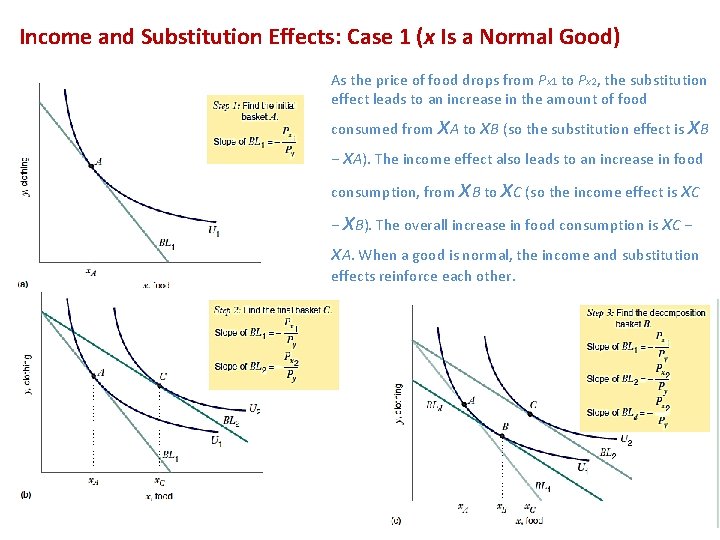
Income and Substitution Effects: (x Is a Normal Good) Back to 46 Back to 45 Figure shows three optimal choice diagrams that illustrate the steps involved in finding the substitution effect associated with this price change.

Income and Substitution Effects: Case 1 (x Is a Normal Good) As the price of food drops from Px 1 to Px 2, the substitution effect leads to an increase in the amount of food x x consumed from A to x. B (so the substitution effect is B − x. A). The income effect also leads to an increase in food x x consumption, from B to C (so the income effect is x. C x − B). The overall increase in food consumption is x. C − x. A. When a good is normal, the income and substitution effects reinforce each other.

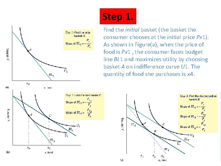
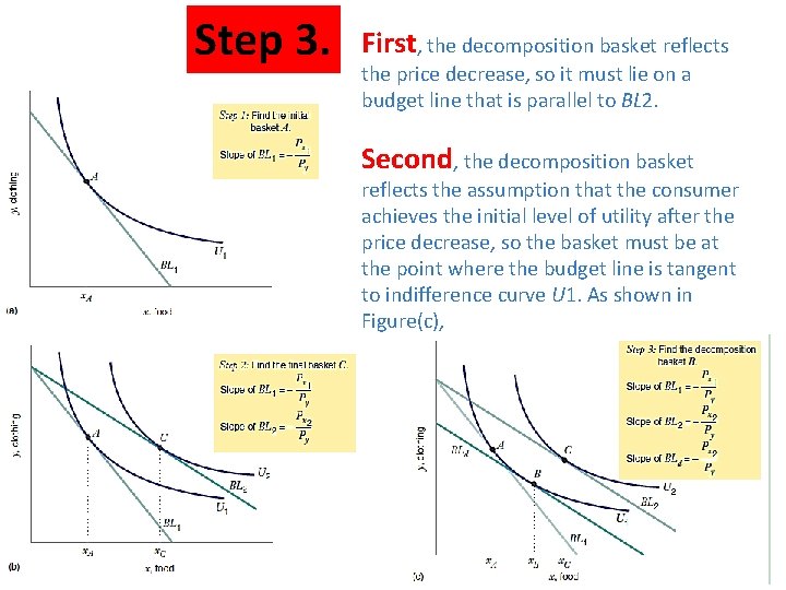
Step 1. Find the initial basket (the basket the consumer chooses at the initial price Px 1). As shown in Figure(a), when the price of food is Px 1 , the consumer faces budget line BL 1 and maximizes utility by choosing basket A on indifference curve U 1. The quantity of food she purchases is x. A.

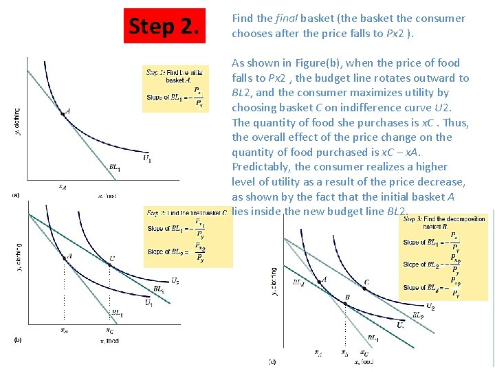
Step 2. Find the final basket (the basket the consumer chooses after the price falls to Px 2 ). As shown in Figure(b), when the price of food falls to Px 2 , the budget line rotates outward to BL 2, and the consumer maximizes utility by choosing basket C on indifference curve U 2. The quantity of food she purchases is x. C. Thus, the overall effect of the price change on the quantity of food purchased is x. C − x. A. Predictably, the consumer realizes a higher level of utility as a result of the price decrease, as shown by the fact that the initial basket A lies inside the new budget line BL 2.

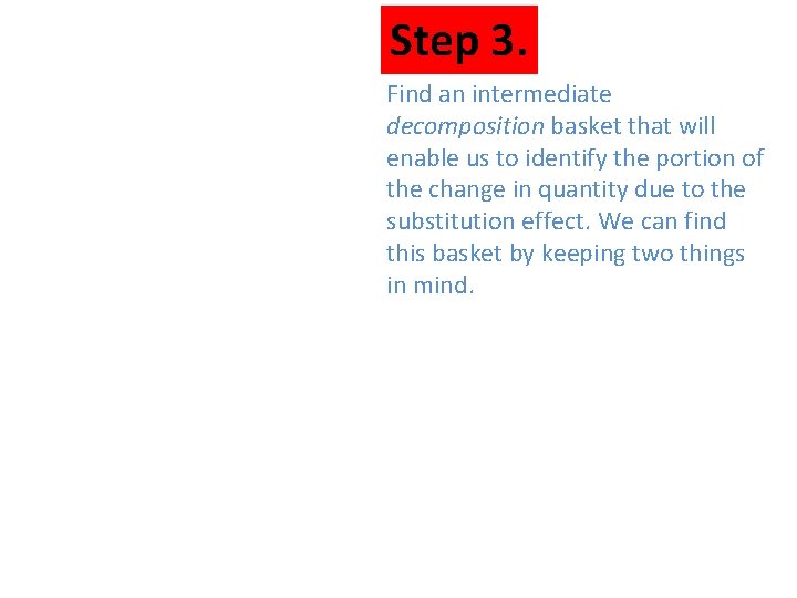
Step 3. Find an intermediate decomposition basket that will enable us to identify the portion of the change in quantity due to the substitution effect. We can find this basket by keeping two things in mind.

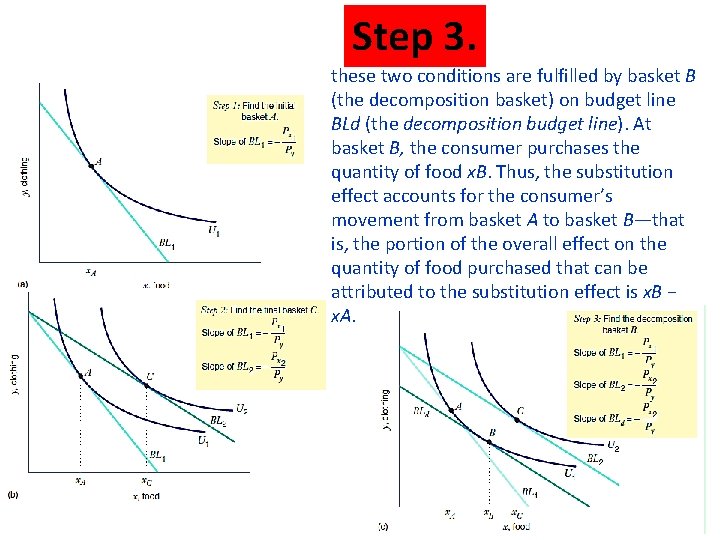
Step 3. First, the decomposition basket reflects the price decrease, so it must lie on a budget line that is parallel to BL 2. Second, the decomposition basket reflects the assumption that the consumer achieves the initial level of utility after the price decrease, so the basket must be at the point where the budget line is tangent to indifference curve U 1. As shown in Figure(c),

Step 3. these two conditions are fulfilled by basket B (the decomposition basket) on budget line BLd (the decomposition budget line). At basket B, the consumer purchases the quantity of food x. B. Thus, the substitution effect accounts for the consumer’s movement from basket A to basket B—that is, the portion of the overall effect on the quantity of food purchased that can be attributed to the substitution effect is x. B − x. A.

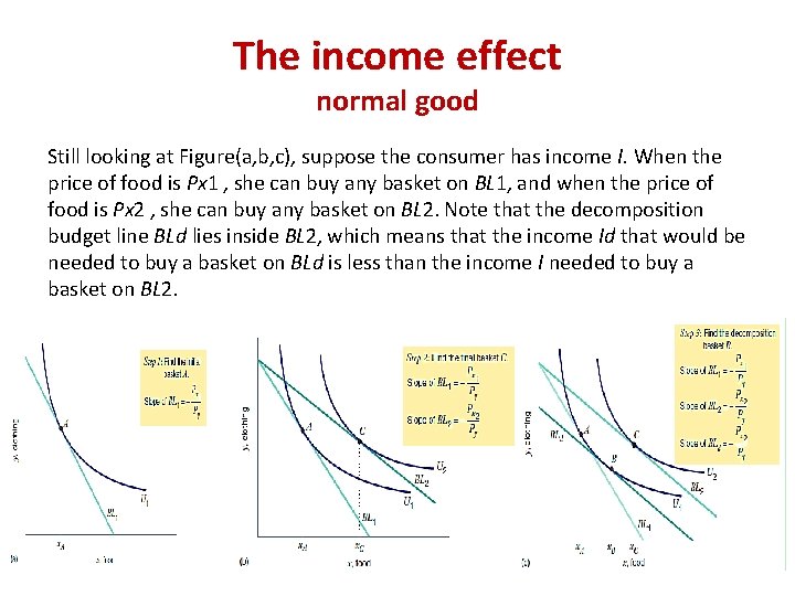
The income effect normal good Still looking at Figure(a, b, c), suppose the consumer has income I. When the price of food is Px 1 , she can buy any basket on BL 1, and when the price of food is Px 2 , she can buy any basket on BL 2. Note that the decomposition budget line BLd lies inside BL 2, which means that the income Id that would be needed to buy a basket on BLd is less than the income I needed to buy a basket on BL 2.

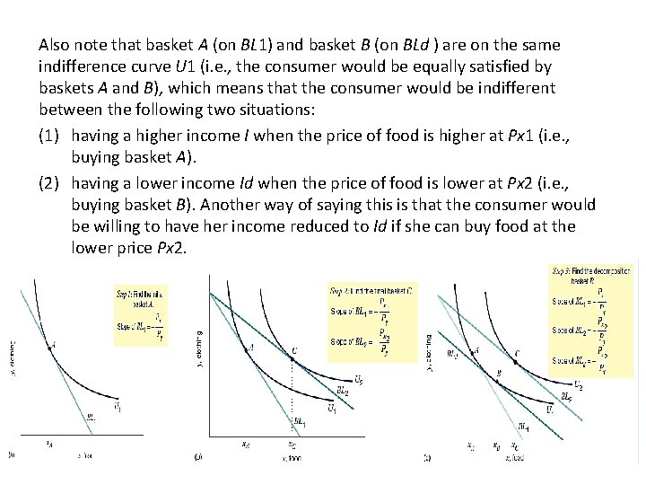
Also note that basket A (on BL 1) and basket B (on BLd ) are on the same indifference curve U 1 (i. e. , the consumer would be equally satisfied by baskets A and B), which means that the consumer would be indifferent between the following two situations: (1) having a higher income I when the price of food is higher at Px 1 (i. e. , buying basket A). (2) having a lower income Id when the price of food is lower at Px 2 (i. e. , buying basket B). Another way of saying this is that the consumer would be willing to have her income reduced to Id if she can buy food at the lower price Px 2.

The income effect, the change in the amount of a good consumed as the consumer’s utility changes. In the example illustrated by Figure in slide 36, the movement from basket A to basket B (i. e. , the movement due to the substitution effect) doesn’t involve any change in utility, and as we have just seen, we can view this movement as the result of a reduction in income from I to Id as the price falls from Px 1 to Px 2

In reality, however, the consumer’s income doesn’t fall when the price of food decreases, so her level of utility increases, and we account for this by “restoring” the “lost” income. When we do this, the budget line shifts from BLd to BL 2, and the consumer’s optimal basket shifts from basket B (on BLd ) to basket C (on BL 2). Thus, the income effect accounts for the consumer’s movement from the decomposition basket B to the final basket C—that is, the portion of the overall effect on the quantity of food purchased that can be attributed to the income effect is x. C − x. B. Graph 36

In sum, when the price of food falls from Px 1 to Px 2 , the total change on food consumption is (x. C − x. A). This can be decomposed into the substitution effect (x. B − x. A) and the income effect (x. C − x. B ). Graph 36 When we add the substitution effect and the income effect, we get the total change in consumption.

Abstract As we noted, the graphs are drawn for the case in which food is a normal good. As the price of food falls, the income effect leads to an increase in food consumption. Also, because the marginal rate of substitution is diminishing, the substitution effect leads to increased food consumption as well. Thus, the income and substitution effects work in the same direction. The demand curve for food will be downward sloping because the quantity of food purchased will increase when the price of food falls. (Similarly, if the price of food were to rise, both effects would be negative. At a higher price of food, the consumer would buy less food. )

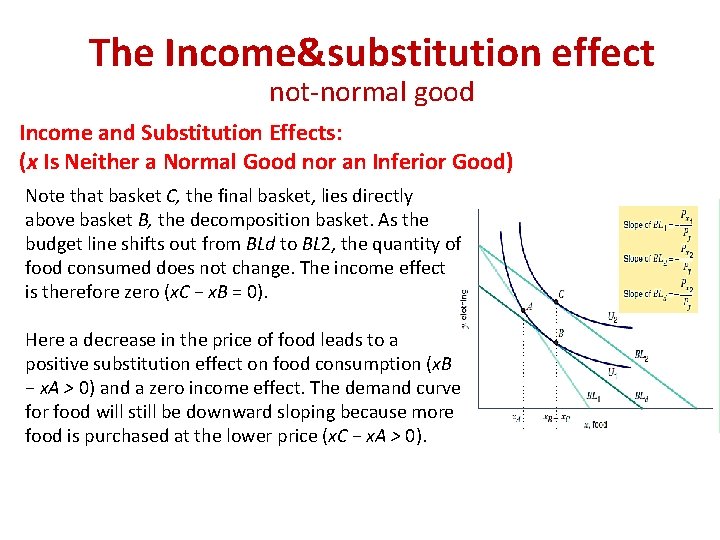
The Income&substitution effect not-normal good Income and Substitution Effects: (x Is Neither a Normal Good nor an Inferior Good) Note that basket C, the final basket, lies directly above basket B, the decomposition basket. As the budget line shifts out from BLd to BL 2, the quantity of food consumed does not change. The income effect is therefore zero (x. C − x. B = 0). Here a decrease in the price of food leads to a positive substitution effect on food consumption (x. B − x. A > 0) and a zero income effect. The demand curve for food will still be downward sloping because more food is purchased at the lower price (x. C − x. A > 0).

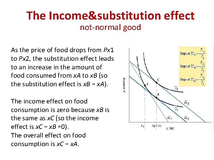
The Income&substitution effect not-normal good As the price of food drops from Px 1 to Px 2, the substitution effect leads to an increase in the amount of food consumed from x. A to x. B (so the substitution effect is x. B − x. A). The income effect on food consumption is zero because x. B is the same as x. C (so the income effect is x. C − x. B =0). The overall effect on food consumption is x. C − x. A.

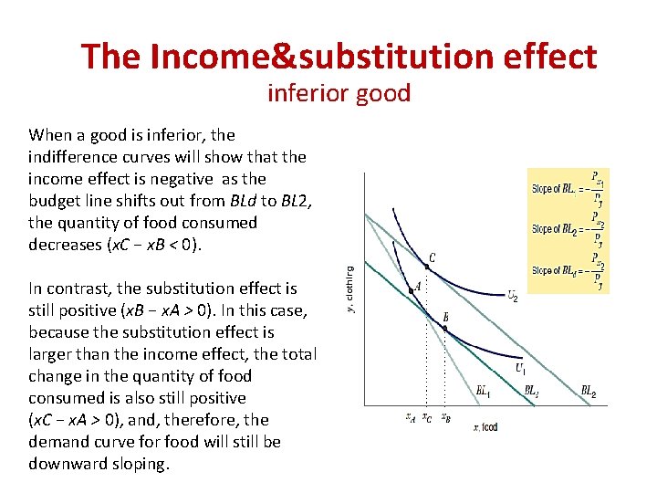
The Income&substitution effect inferior good When a good is inferior, the indifference curves will show that the income effect is negative as the budget line shifts out from BLd to BL 2, the quantity of food consumed decreases (x. C − x. B < 0). In contrast, the substitution effect is still positive (x. B − x. A > 0). In this case, because the substitution effect is larger than the income effect, the total change in the quantity of food consumed is also still positive (x. C − x. A > 0), and, therefore, the demand curve for food will still be downward sloping.

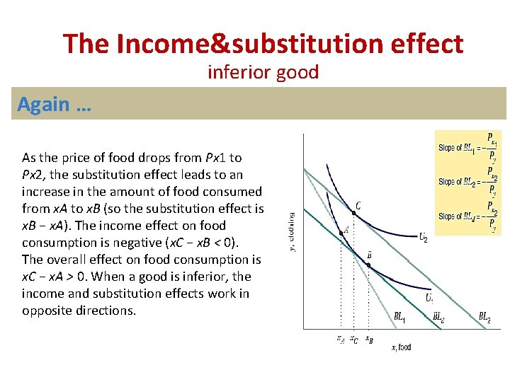
The Income&substitution effect inferior good Again … As the price of food drops from Px 1 to Px 2, the substitution effect leads to an increase in the amount of food consumed from x. A to x. B (so the substitution effect is x. B − x. A). The income effect on food consumption is negative (x. C − x. B < 0). The overall effect on food consumption is x. C − x. A > 0. When a good is inferior, the income and substitution effects work in opposite directions.

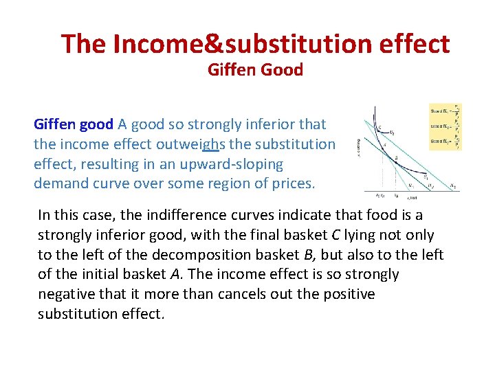
The Income&substitution effect Giffen Good Giffen good A good so strongly inferior that the income effect outweighs the substitution effect, resulting in an upward-sloping demand curve over some region of prices. In this case, the indifference curves indicate that food is a strongly inferior good, with the final basket C lying not only to the left of the decomposition basket B, but also to the left of the initial basket A. The income effect is so strongly negative that it more than cancels out the positive substitution effect.

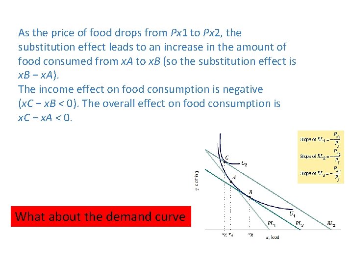
As the price of food drops from Px 1 to Px 2, the substitution effect leads to an increase in the amount of food consumed from x. A to x. B (so the substitution effect is x. B − x. A). The income effect on food consumption is negative (x. C − x. B < 0). The overall effect on food consumption is x. C − x. A < 0. What about the demand curve

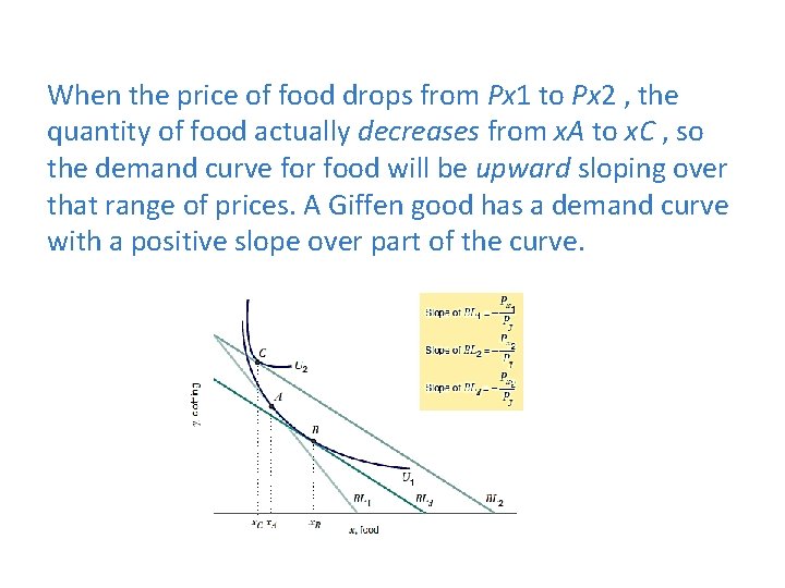
When the price of food drops from Px 1 to Px 2 , the quantity of food actually decreases from x. A to x. C , so the demand curve for food will be upward sloping over that range of prices. A Giffen good has a demand curve with a positive slope over part of the curve.

Problem A consumer who purchases two goods, food and clothing. He has the utility function U(x, y) = xy, where x denotes the amount of food consumed and y the amount of clothing. His marginal utilities are MUx = y and MUy = x. Now suppose that he has an income of $72 per week and that the price of clothing is Py = $1 per unit. Suppose that the price of food is initially Px 1 = $9 per unit, and that the price subsequently falls to Px 2= $4 per unit. Find the numerical values of the income and substitution effects on food consumption, and graph the results.

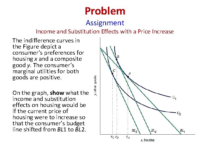
Problem Assignment Income and Substitution Effects with a Price Increase The indifference curves in the Figure depict a consumer’s preferences for housing x and a composite good y. The consumer’s marginal utilities for both goods are positive. On the graph, show what the income and substitution effects on housing would be if the current price of housing were to increase so that the consumer’s budget line shifted from BL 1 to BL 2.

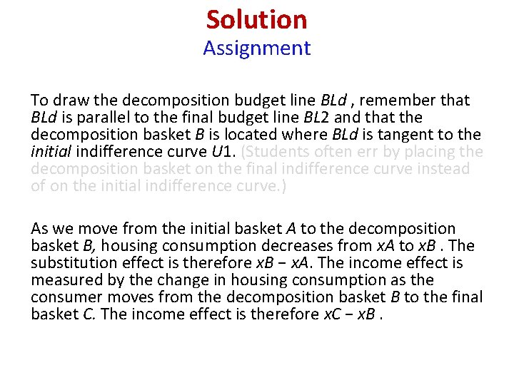
Solution Assignment To draw the decomposition budget line BLd , remember that BLd is parallel to the final budget line BL 2 and that the decomposition basket B is located where BLd is tangent to the initial indifference curve U 1. (Students often err by placing the decomposition basket on the final indifference curve instead of on the initial indifference curve. ) As we move from the initial basket A to the decomposition basket B, housing consumption decreases from x. A to x. B. The substitution effect is therefore x. B − x. A. The income effect is measured by the change in housing consumption as the consumer moves from the decomposition basket B to the final basket C. The income effect is therefore x. C − x. B.

consumer surplus • Next Lecturer