Supply and Demand 1 Demand n A demand

Supply and Demand 1

Demand n A demand curve shows the amount of a good consumers wish to purchase at specified prices. n Demand curve is downward sloping n Demand refers to the whole schedule of prices and quantity demanded. n Quantity demanded is the amount demanded at a particular price.

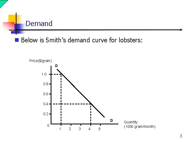
Demand n Below is Smith’s demand curve for lobsters: Price($/gram) D 1. 0 0. 8 0. 6 0. 4 0. 2 D 0 1 2 3 4 5 Quantity (1000 gram/month) 3

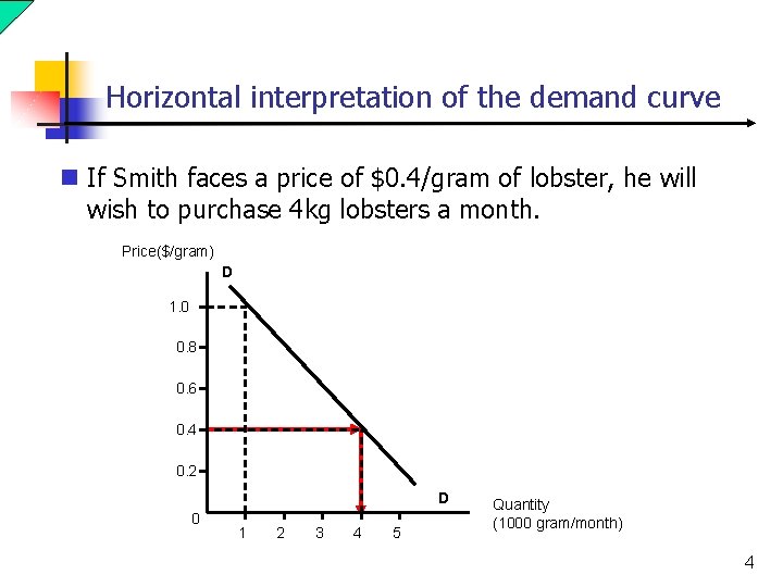
Horizontal interpretation of the demand curve n If Smith faces a price of $0. 4/gram of lobster, he will wish to purchase 4 kg lobsters a month. Price($/gram) D 1. 0 0. 8 0. 6 0. 4 0. 2 D 0 1 2 3 4 5 Quantity (1000 gram/month) 4

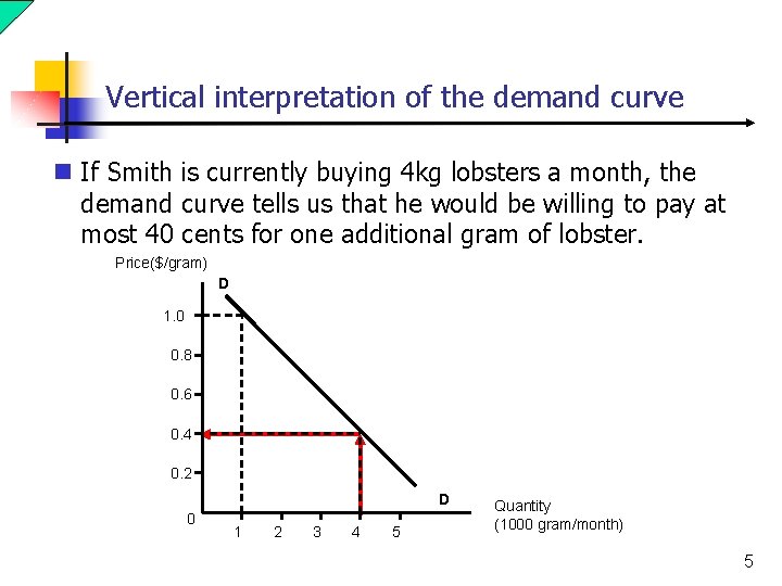
Vertical interpretation of the demand curve n If Smith is currently buying 4 kg lobsters a month, the demand curve tells us that he would be willing to pay at most 40 cents for one additional gram of lobster. Price($/gram) D 1. 0 0. 8 0. 6 0. 4 0. 2 D 0 1 2 3 4 5 Quantity (1000 gram/month) 5

Supply n A supply curve shows the amount of some good sellers are willing to offer at various prices. n In general, supply curve is upward sloping. n Supply refers to the whole schedule of prices and quantity supplied. n Quantity supplied is the amount supplied at a particular price.

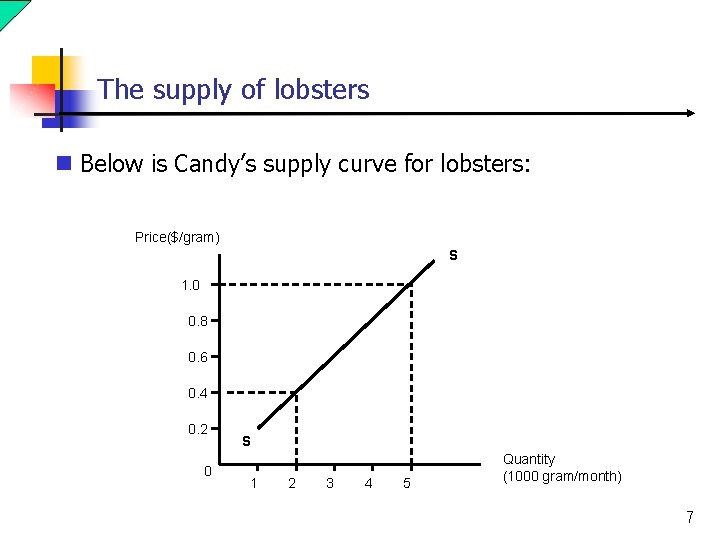
The supply of lobsters n Below is Candy’s supply curve for lobsters: Price($/gram) S 1. 0 0. 8 0. 6 0. 4 0. 2 0 S 1 2 3 4 5 Quantity (1000 gram/month) 7

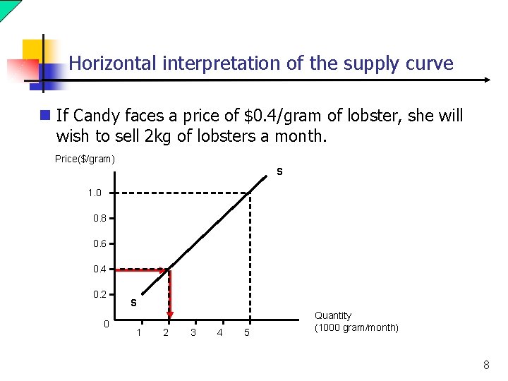
Horizontal interpretation of the supply curve n If Candy faces a price of $0. 4/gram of lobster, she will wish to sell 2 kg of lobsters a month. Price($/gram) S 1. 0 0. 8 0. 6 0. 4 0. 2 0 S 1 2 3 4 5 Quantity (1000 gram/month) 8

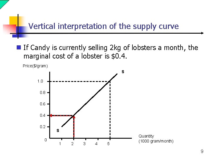
Vertical interpretation of the supply curve n If Candy is currently selling 2 kg of lobsters a month, the marginal cost of a lobster is $0. 4. Price($/gram) S 1. 0 0. 8 0. 6 0. 4 0. 2 0 S 1 2 3 4 5 Quantity (1000 gram/month) 9

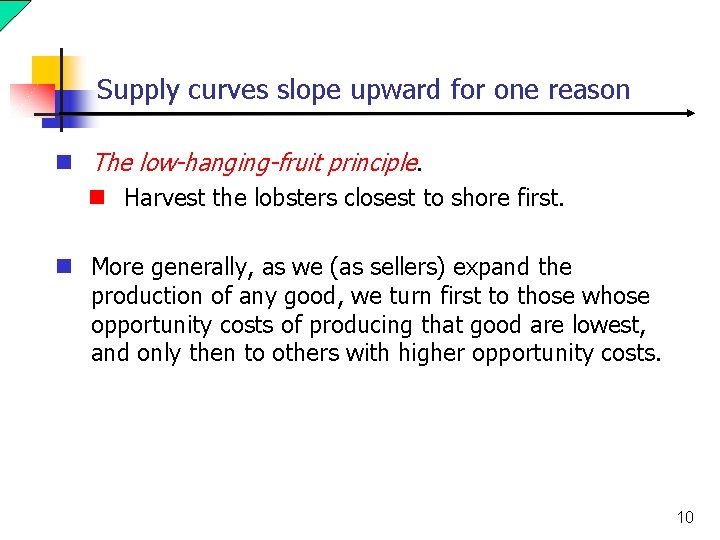
Supply curves slope upward for one reason n The low-hanging-fruit principle. n Harvest the lobsters closest to shore first. n More generally, as we (as sellers) expand the production of any good, we turn first to those whose opportunity costs of producing that good are lowest, and only then to others with higher opportunity costs. 10

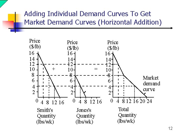
Adding Individual Demand Curves To Get Market Demand Curves (Horizontal Addition) n Suppose that there only two buyers—Smith and Jones— in the market for lobsters, and that their demand curves are as shown in the following slide. n To construct the market demand curve for lobsters, we simply announce a sequence of prices and then add the quantity demanded by each buyer at each price to obtain the total quantity demanded. 11

Adding Individual Demand Curves To Get Market Demand Curves (Horizontal Addition) Price ($/lb) 16 14 12 10 8 6 4 2 Price ($/lb) 16 14 12 + = 10 8 6 4 2 0 4 8 12 16 Smith's Jones's Quantity (lbs/wk) Price ($/lb) 16 14 12 10 8 Market 6 demand 4 curve 2 0 4 8 12 16 20 24 Total Quantity (lbs/wk) 12

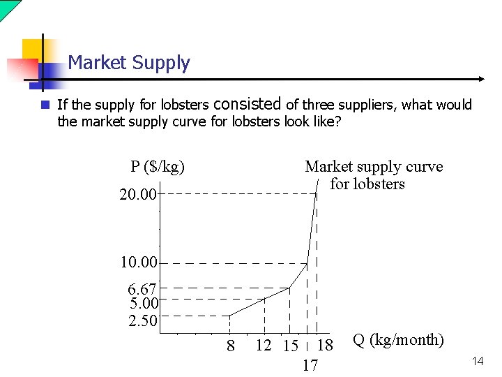
Market Supply n Similar to the market demand, the quantity that corresponds to any given price on the market supply curve is the horizontal summation of the quantities supplied at that price by all individual sellers in the market. 13

Market Supply n If the supply for lobsters consisted of three suppliers, what would the market supply curve for lobsters look like? P ($/kg) Market supply curve for lobsters 20. 00 10. 00 6. 67 5. 00 2. 50 8 12 15 18 17 Q (kg/month) 14

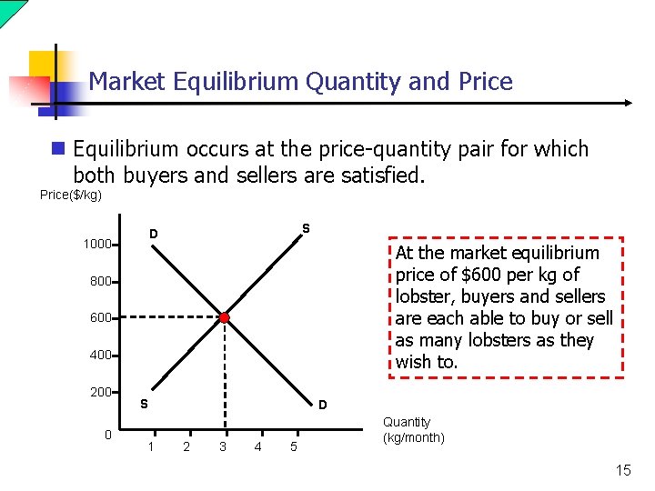
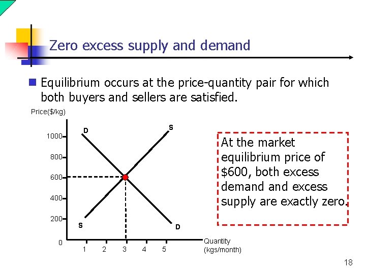
Market Equilibrium Quantity and Price n Equilibrium occurs at the price-quantity pair for which both buyers and sellers are satisfied. Price($/kg) S D 1000 At the market equilibrium price of $600 per kg of lobster, buyers and sellers are each able to buy or sell as many lobsters as they wish to. 800 600 400 200 0 S 1 D 2 3 4 5 Quantity (kg/month) 15

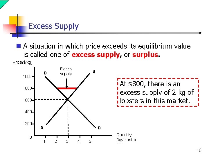
Excess Supply n A situation in which price exceeds its equilibrium value is called one of excess supply, or surplus. Price($/kg) Excess supply D 1000 S At $800, there is an excess supply of 2 kg of lobsters in this market. 800 600 400 200 0 S 1 D 2 3 4 5 Quantity (kg/month) 16

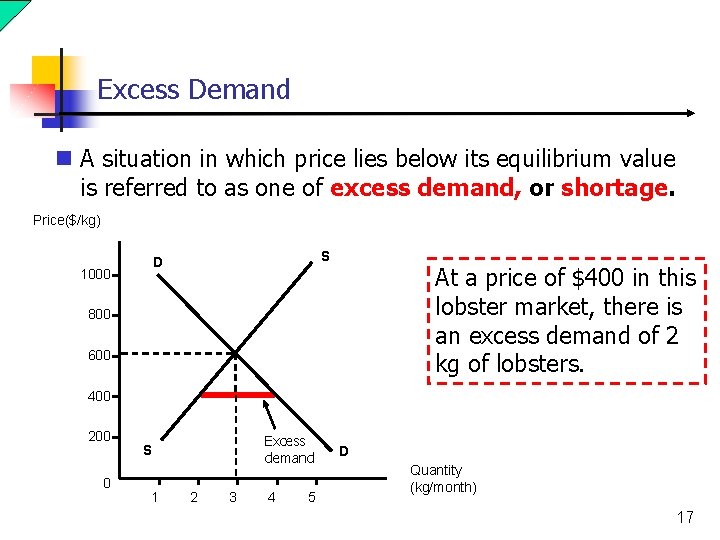
Excess Demand n A situation in which price lies below its equilibrium value is referred to as one of excess demand, or shortage. Price($/kg) S D 1000 At a price of $400 in this lobster market, there is an excess demand of 2 kg of lobsters. 800 600 400 200 0 Excess demand S 1 2 3 4 5 D Quantity (kg/month) 17

Zero excess supply and demand n Equilibrium occurs at the price-quantity pair for which both buyers and sellers are satisfied. Price($/kg) S D 1000 At the market equilibrium price of $600, both excess demand excess supply are exactly zero. 800 600 400 200 0 S 1 D 2 3 4 5 Quantity (kgs/month) 18

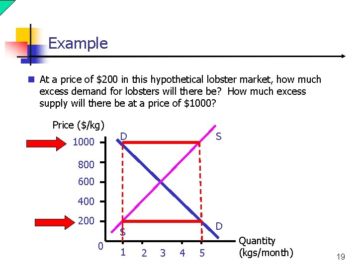
Example n At a price of $200 in this hypothetical lobster market, how much excess demand for lobsters will there be? How much excess supply will there be at a price of $1000? Price ($/kg) 1000 D S 800 600 400 200 D S 0 1 2 3 4 5 Quantity (kgs/month) 19

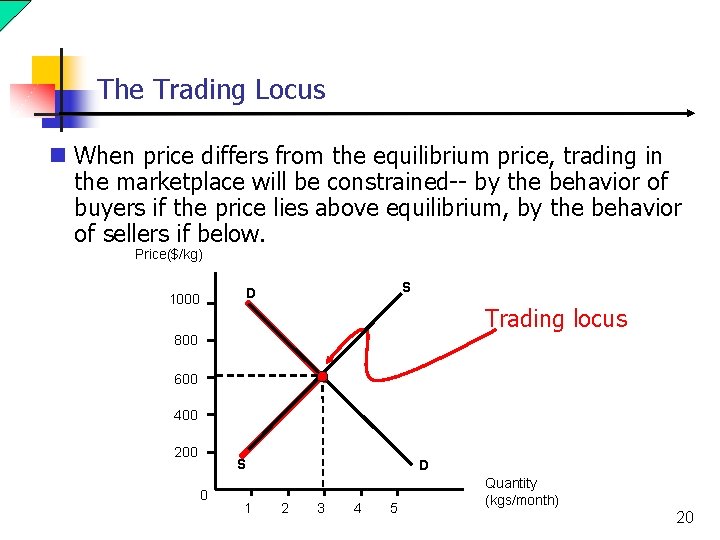
The Trading Locus n When price differs from the equilibrium price, trading in the marketplace will be constrained-- by the behavior of buyers if the price lies above equilibrium, by the behavior of sellers if below. Price($/kg) S D 1000 Trading locus 800 600 400 200 S 0 1 D 2 3 4 5 Quantity (kgs/month) 20

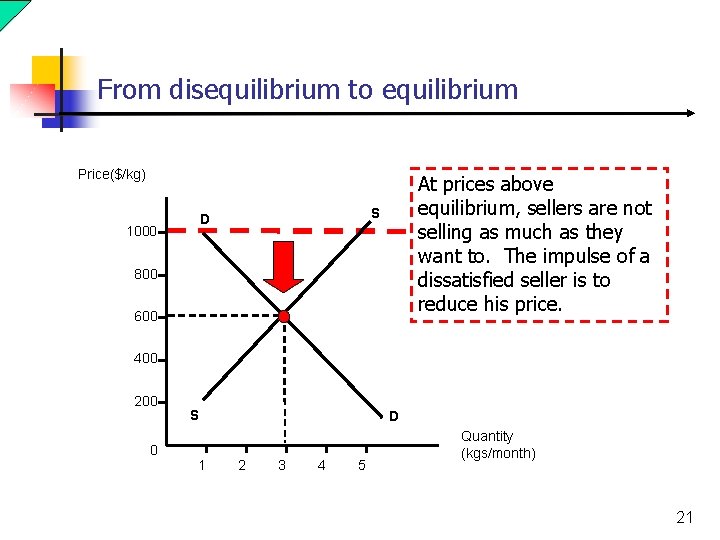
From disequilibrium to equilibrium Price($/kg) S D 1000 At prices above equilibrium, sellers are not selling as much as they want to. The impulse of a dissatisfied seller is to reduce his price. 800 600 400 200 0 S 1 D 2 3 4 5 Quantity (kgs/month) 21

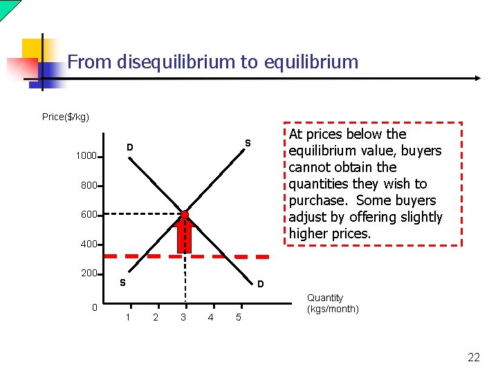
From disequilibrium to equilibrium Price($/kg) D 1000 At prices below the equilibrium value, buyers cannot obtain the quantities they wish to purchase. Some buyers adjust by offering slightly higher prices. S 800 600 400 200 0 S 1 D 2 3 4 5 Quantity (kgs/month) 22

From disequilibrium to equilibrium n An extraordinary feature of this equilibrating process is that no one consciously plans or directs it. n The actual steps that consumers and producers must take to move toward equilibrium are often indescribably complex. n Suppliers looking to expand their operations, for example, must choose from a bewilderingly large menu of equipment options. n Buyers, for their part, face literally millions of choices about how to spend their money. 23

From disequilibrium to equilibrium n And yet the adjustment toward equilibrium results more or less automatically from the natural reactions of selfinterested individuals facing either surpluses or shortages. n How long does it take to arrive at equilibrium from an disequilibrium? n “The market can stay irrational a lot longer than you can stay solvent!” (John M. Keynes, referring to financial markets) 24

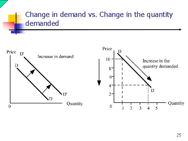
Change in demand vs. Change in the quantity demanded 25

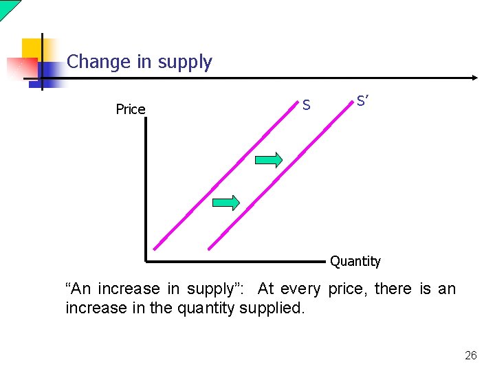
Change in supply Price S S’ Quantity “An increase in supply”: At every price, there is an increase in the quantity supplied. 26

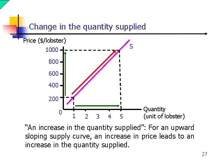
Change in the quantity supplied Price ($/lobster) S 1000 800 600 400 200 0 1 2 3 4 5 Quantity (unit of lobster) “An increase in the quantity supplied”: For an upward sloping supply curve, an increase in price leads to an increase in the quantity supplied. 27

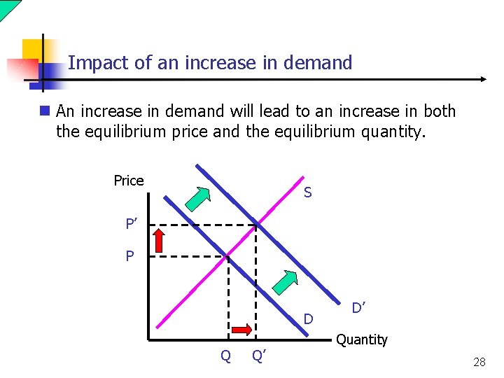
Impact of an increase in demand n An increase in demand will lead to an increase in both the equilibrium price and the equilibrium quantity. Price S P’ P D Q Q’ D’ Quantity 28

Impact of a decrease in demand n A decrease in demand will lead to a reduction in both the equilibrium price and the equilibrium quantity. Price S P P’ D’ Q’ Q D Quantity 29

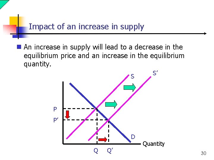
Impact of an increase in supply n An increase in supply will lead to a decrease in the equilibrium price and an increase in the equilibrium quantity. S S’ P P’ D Q Q’ Quantity 30

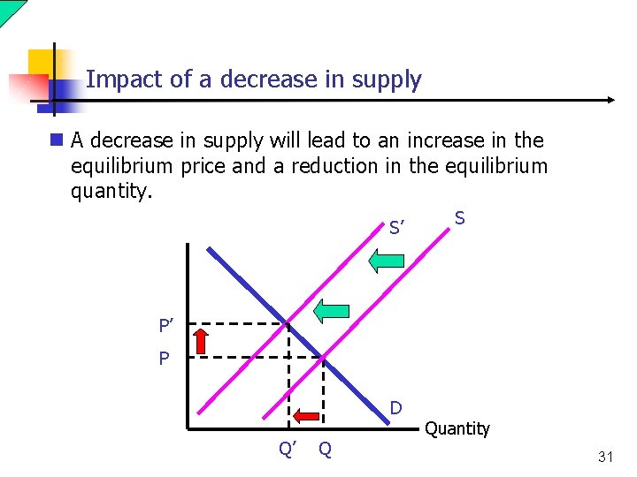
Impact of a decrease in supply n A decrease in supply will lead to an increase in the equilibrium price and a reduction in the equilibrium quantity. S’ S P’ P D Q’ Q Quantity 31

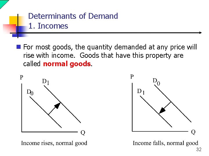
Determinants of Demand 1. Incomes n For most goods, the quantity demanded at any price will rise with income. Goods that have this property are called normal goods. 32

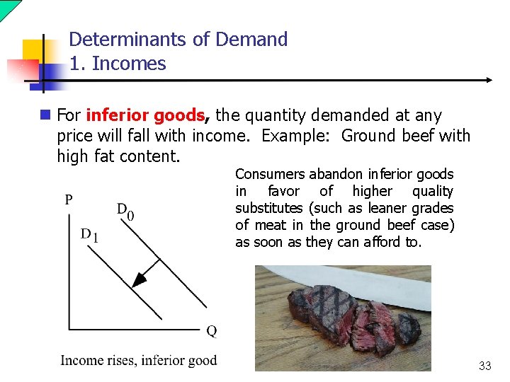
Determinants of Demand 1. Incomes n For inferior goods, the quantity demanded at any price will fall with income. Example: Ground beef with high fat content. Consumers abandon inferior goods in favor of higher quality substitutes (such as leaner grades of meat in the ground beef case) as soon as they can afford to. 33

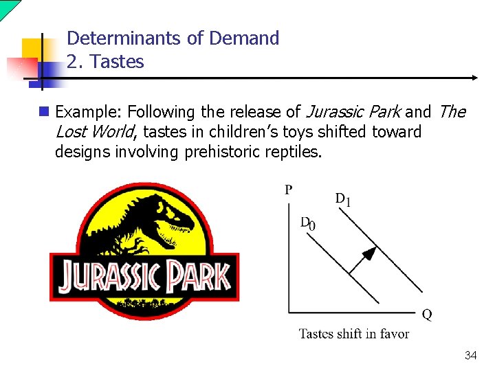
Determinants of Demand 2. Tastes n Example: Following the release of Jurassic Park and The Lost World, tastes in children’s toys shifted toward designs involving prehistoric reptiles. 34

Determinants of Demand 3. Prices of substitutes 35

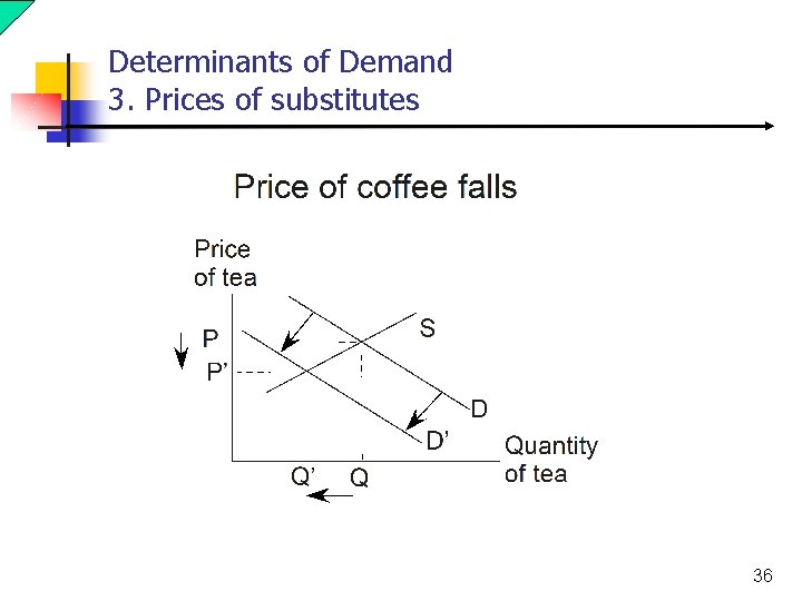
Determinants of Demand 3. Prices of substitutes 36

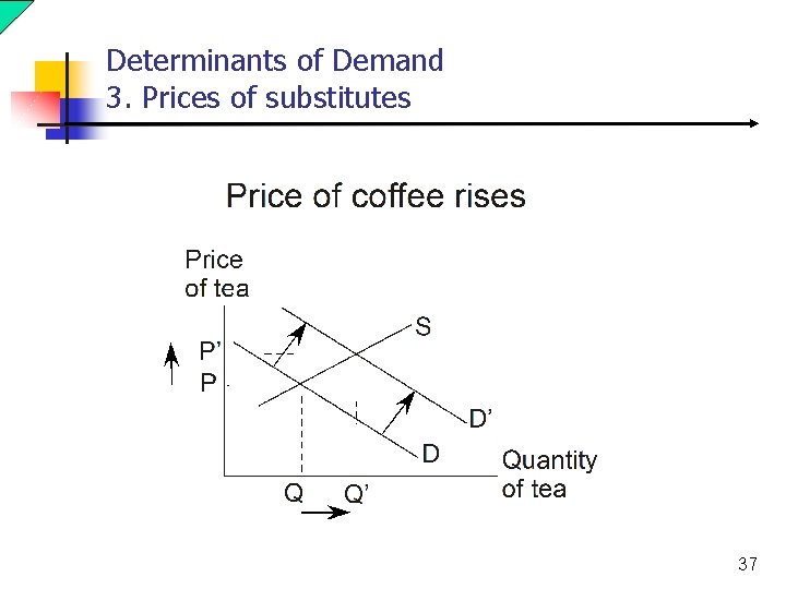
Determinants of Demand 3. Prices of substitutes 37

Determinants of Demand 4. Prices of complements 38

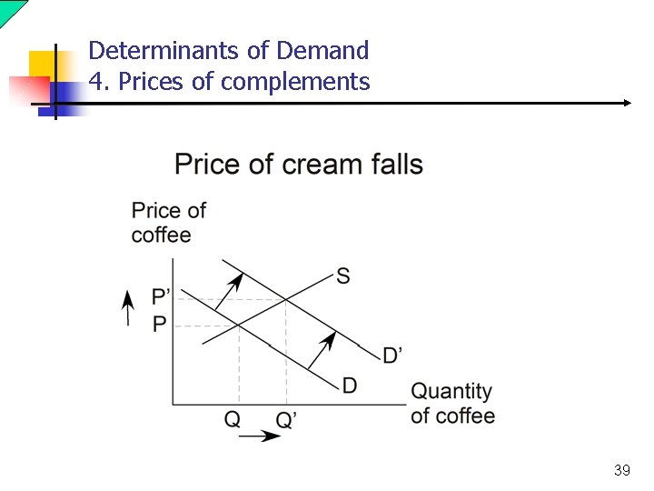
Determinants of Demand 4. Prices of complements 39

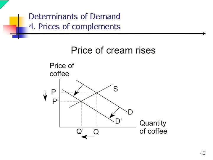
Determinants of Demand 4. Prices of complements 40

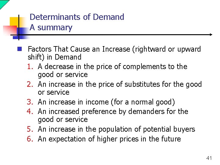
Determinants of Demand A summary n Factors That Cause an Increase (rightward or upward shift) in Demand 1. A decrease in the price of complements to the good or service 2. An increase in the price of substitutes for the good or service 3. An increase in income (for a normal good) 4. An increased preference by demanders for the good or service 5. An increase in the population of potential buyers 6. An expectation of higher prices in the future 41

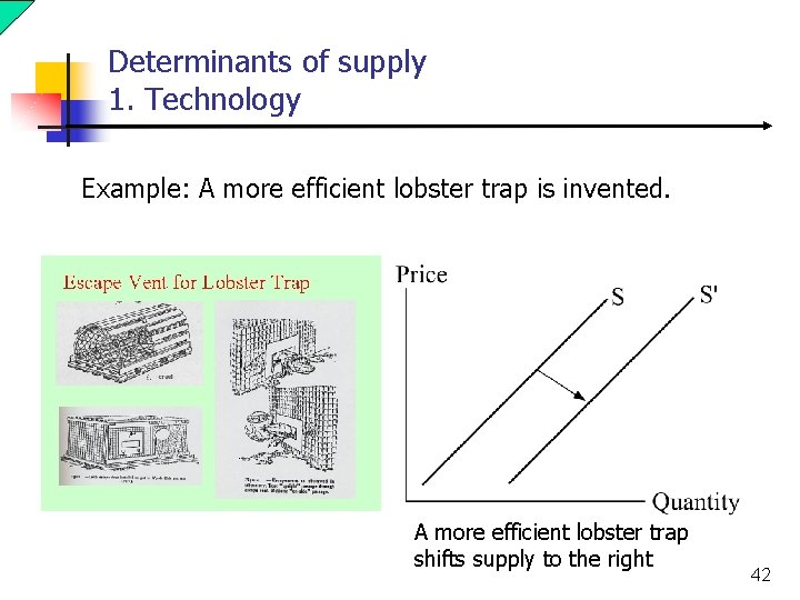
Determinants of supply 1. Technology Example: A more efficient lobster trap is invented. A more efficient lobster trap shifts supply to the right 42

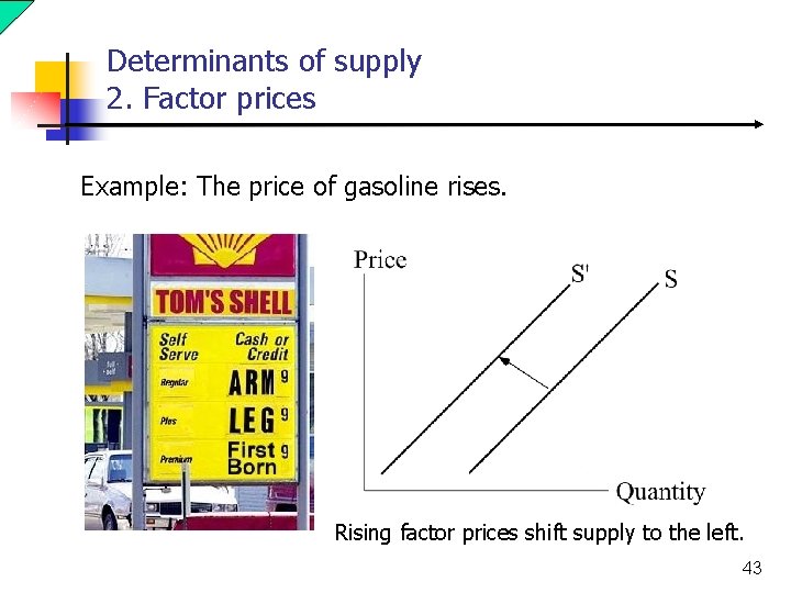
Determinants of supply 2. Factor prices Example: The price of gasoline rises. Rising factor prices shift supply to the left. 43

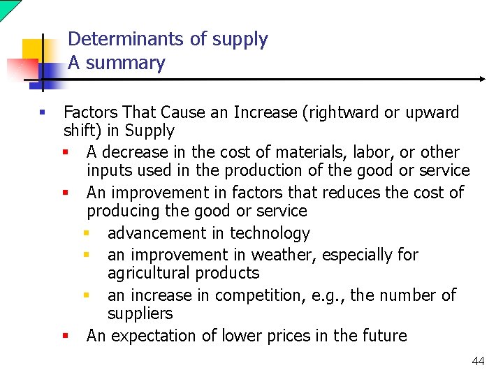
Determinants of supply A summary § Factors That Cause an Increase (rightward or upward shift) in Supply § A decrease in the cost of materials, labor, or other inputs used in the production of the good or service § An improvement in factors that reduces the cost of producing the good or service § advancement in technology § an improvement in weather, especially for agricultural products § an increase in competition, e. g. , the number of suppliers § An expectation of lower prices in the future 44

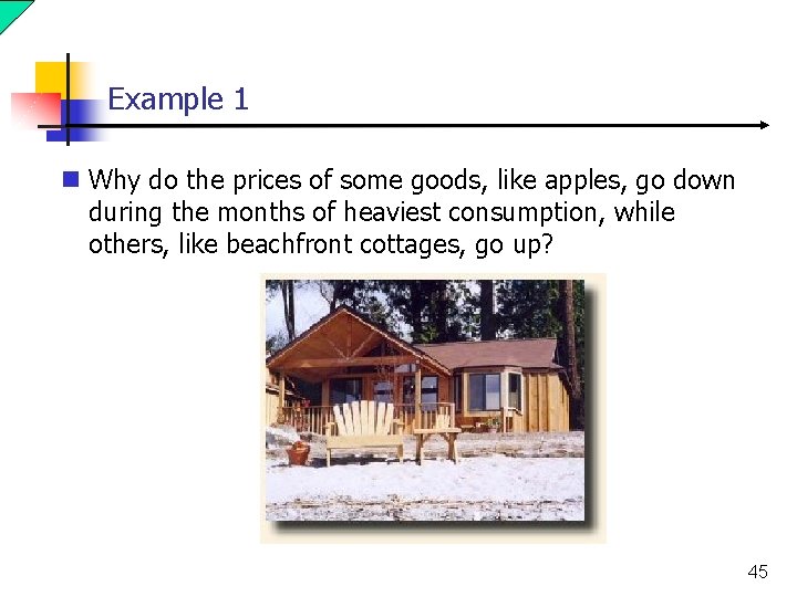
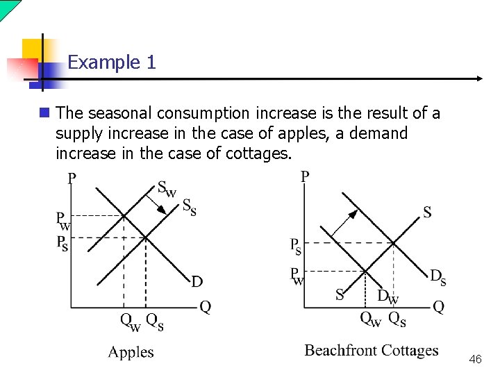
Example 1 n Why do the prices of some goods, like apples, go down during the months of heaviest consumption, while others, like beachfront cottages, go up? 45

Example 1 n The seasonal consumption increase is the result of a supply increase in the case of apples, a demand increase in the case of cottages. 46

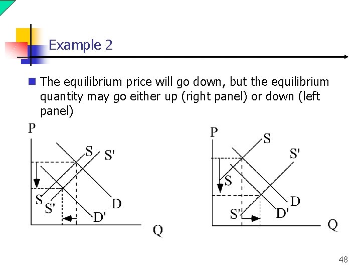
Example 2 n What will happen to the equilibrium price and quantity in the fresh seafood market if both of the following events occur: n a scientific report is issued saying that fish contains mercury, which is toxic to humans; and n the price of diesel fuel falls significantly? 47

Example 2 n The equilibrium price will go down, but the equilibrium quantity may go either up (right panel) or down (left panel) 48

End 49