Statistical Methods for Particle Physics Lecture 4 discovery

Statistical Methods for Particle Physics Lecture 4: discovery, exclusion limits www. pp. rhul. ac. uk/~cowan/stat_aachen. html Graduierten-Kolleg RWTH Aachen 10 -14 February 2014 Glen Cowan Physics Department Royal Holloway, University of London g. cowan@rhul. ac. uk www. pp. rhul. ac. uk/~cowan G. Cowan Aachen 2014 / Statistics for Particle Physics, Lecture 4 1

Outline 1 Probability Definition, Bayes’ theorem, probability densities and their properties, catalogue of pdfs, Monte Carlo 2 Statistical tests general concepts, test statistics, multivariate methods, goodness-of-fit tests 3 Parameter estimation general concepts, maximum likelihood, variance of estimators, least squares 4 Hypothesis tests for discovery and exclusion discovery significance, sensitivity, setting limits 5 Further topics systematic errors, Bayesian methods, MCMC G. Cowan Aachen 2014 / Statistics for Particle Physics, Lecture 4 2

Interval estimation — introduction In addition to a ‘point estimate’ of a parameter we should report an interval reflecting its statistical uncertainty. Desirable properties of such an interval may include: communicate objectively the result of the experiment; have a given probability of containing the true parameter; provide information needed to draw conclusions about the parameter possibly incorporating stated prior beliefs. Often use +/- the estimated standard deviation of the estimator. In some cases, however, this is not adequate: estimate near a physical boundary, e. g. , an observed event rate consistent with zero. We will look briefly at Frequentist and Bayesian intervals. G. Cowan Aachen 2014 / Statistics for Particle Physics, Lecture 4 3

Confidence intervals by inverting a test Frequentist confidence intervals for a parameter can be found by defining a test of the hypothesized value (do this for all ): Specify values of the data that are ‘disfavoured’ by (critical region) such that P(data in critical region) ≤ α for a prespecified α, e. g. , 0. 05 or 0. 1. If data observed in the critical region, reject the value . Now invert the test to define a confidence interval as: set of values that would not be rejected in a test of size α (confidence level is 1 - α ). The interval will cover the true value of with probability ≥ 1 – α. For multiparameter case, θ = (θ 1, . . . , θn), this procedure leads to a “confidence region” (not, in general, rectangular). G. Cowan Aachen 2014 / Statistics for Particle Physics, Lecture 4 4

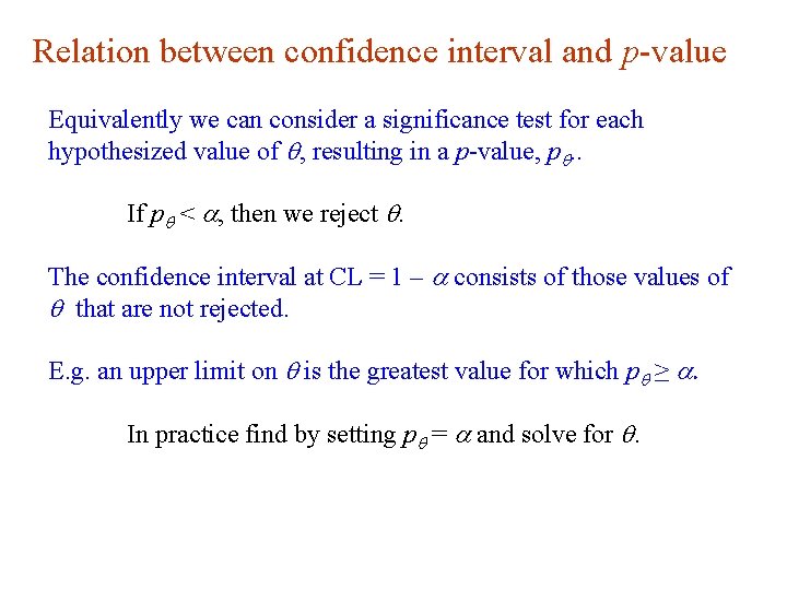
Relation between confidence interval and p-value Equivalently we can consider a significance test for each hypothesized value of , resulting in a p-value, p. . If p < a, then we reject . The confidence interval at CL = 1 – a consists of those values of that are not rejected. E. g. an upper limit on is the greatest value for which p ≥ a. In practice find by setting p = a and solve for . G. Cowan Aachen 2014 / Statistics for Particle Physics, Lecture 4 5

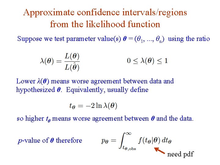
Approximate confidence intervals/regions from the likelihood function Suppose we test parameter value(s) θ = (θ 1, . . . , θn) using the ratio Lower λ(θ) means worse agreement between data and hypothesized θ. Equivalently, usually define so higher tθ means worse agreement between θ and the data. p-value of θ therefore G. Cowan Aachen 2014 / Statistics for Particle Physics, Lecture 4 need pdf 6

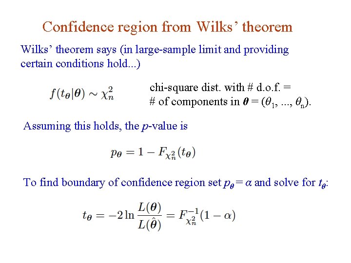
Confidence region from Wilks’ theorem says (in large-sample limit and providing certain conditions hold. . . ) chi-square dist. with # d. o. f. = # of components in θ = (θ 1, . . . , θn). Assuming this holds, the p-value is To find boundary of confidence region set pθ = α and solve for tθ: G. Cowan Aachen 2014 / Statistics for Particle Physics, Lecture 4 7

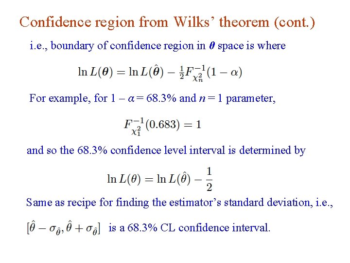
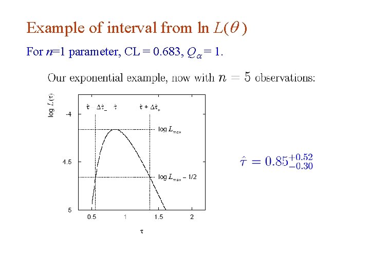
Confidence region from Wilks’ theorem (cont. ) i. e. , boundary of confidence region in θ space is where For example, for 1 – α = 68. 3% and n = 1 parameter, and so the 68. 3% confidence level interval is determined by Same as recipe for finding the estimator’s standard deviation, i. e. , is a 68. 3% CL confidence interval. G. Cowan Aachen 2014 / Statistics for Particle Physics, Lecture 4 8

Example of interval from ln L( ) For n=1 parameter, CL = 0. 683, Qa = 1. G. Cowan Aachen 2014 / Statistics for Particle Physics, Lecture 4 9

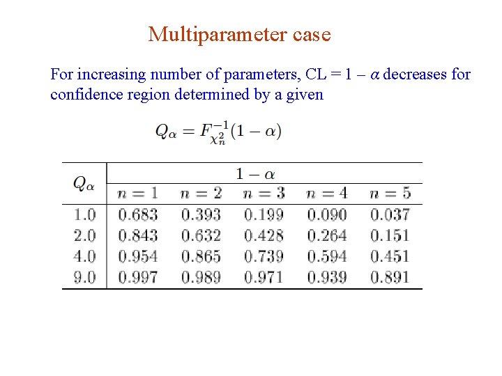
Multiparameter case For increasing number of parameters, CL = 1 – α decreases for confidence region determined by a given G. Cowan Aachen 2014 / Statistics for Particle Physics, Lecture 4 10

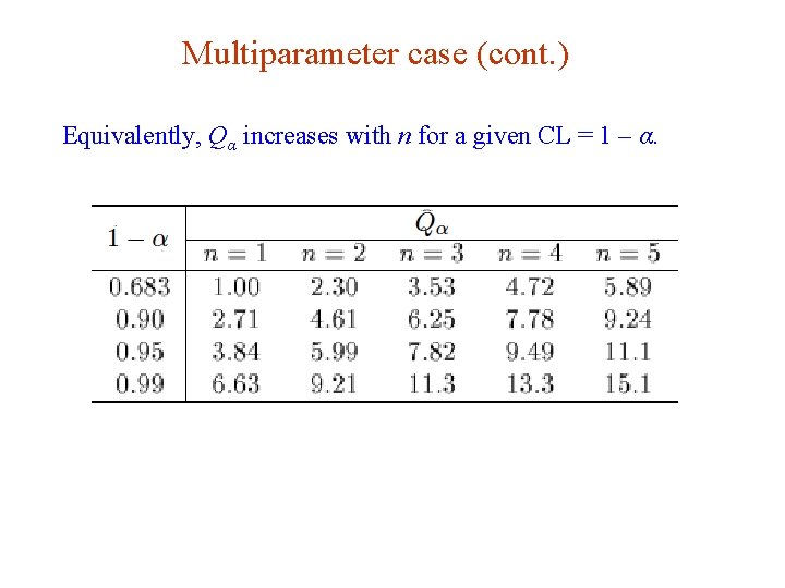
Multiparameter case (cont. ) Equivalently, Qα increases with n for a given CL = 1 – α. G. Cowan Aachen 2014 / Statistics for Particle Physics, Lecture 4 11

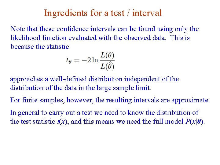
Ingredients for a test / interval Note that these confidence intervals can be found using only the likelihood function evaluated with the observed data. This is because the statistic approaches a well-defined distribution independent of the distribution of the data in the large sample limit. For finite samples, however, the resulting intervals are approximate. In general to carry out a test we need to know the distribution of the test statistic t(x), and this means we need the full model P(x|θ). G. Cowan Aachen 2014 / Statistics for Particle Physics, Lecture 4 12

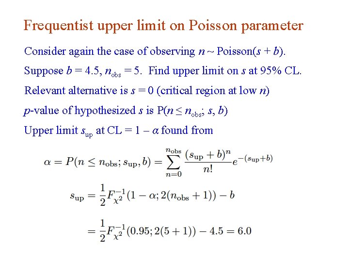
Frequentist upper limit on Poisson parameter Consider again the case of observing n ~ Poisson(s + b). Suppose b = 4. 5, nobs = 5. Find upper limit on s at 95% CL. Relevant alternative is s = 0 (critical region at low n) p-value of hypothesized s is P(n ≤ nobs; s, b) Upper limit sup at CL = 1 – α found from G. Cowan Aachen 2014 / Statistics for Particle Physics, Lecture 4 13

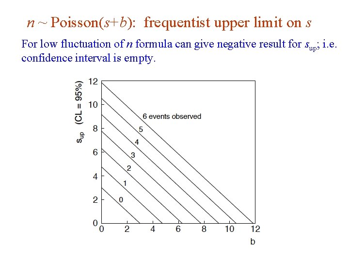
n ~ Poisson(s+b): frequentist upper limit on s For low fluctuation of n formula can give negative result for sup; i. e. confidence interval is empty. G. Cowan Aachen 2014 / Statistics for Particle Physics, Lecture 4 14

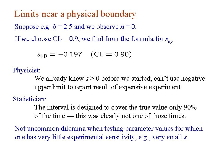
Limits near a physical boundary Suppose e. g. b = 2. 5 and we observe n = 0. If we choose CL = 0. 9, we find from the formula for sup Physicist: We already knew s ≥ 0 before we started; can’t use negative upper limit to report result of expensive experiment! Statistician: The interval is designed to cover the true value only 90% of the time — this was clearly not one of those times. Not uncommon dilemma when testing parameter values for which one has very little experimental sensitivity, e. g. , very small s. G. Cowan Aachen 2014 / Statistics for Particle Physics, Lecture 4 15

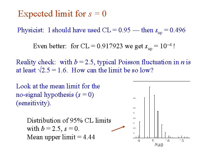
Expected limit for s = 0 Physicist: I should have used CL = 0. 95 — then sup = 0. 496 Even better: for CL = 0. 917923 we get sup = 10 -4 ! Reality check: with b = 2. 5, typical Poisson fluctuation in n is at least √ 2. 5 = 1. 6. How can the limit be so low? Look at the mean limit for the no-signal hypothesis (s = 0) (sensitivity). Distribution of 95% CL limits with b = 2. 5, s = 0. Mean upper limit = 4. 44 G. Cowan Aachen 2014 / Statistics for Particle Physics, Lecture 4 16

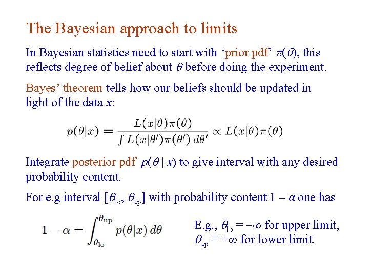
The Bayesian approach to limits In Bayesian statistics need to start with ‘prior pdf’ p( ), this reflects degree of belief about before doing the experiment. Bayes’ theorem tells how our beliefs should be updated in light of the data x: Integrate posterior pdf p( | x) to give interval with any desired probability content. For e. g interval [ lo, up] with probability content 1 – α one has E. g. , lo = -∞ for upper limit, up = +∞ for lower limit. G. Cowan Aachen 2014 / Statistics for Particle Physics, Lecture 4 17

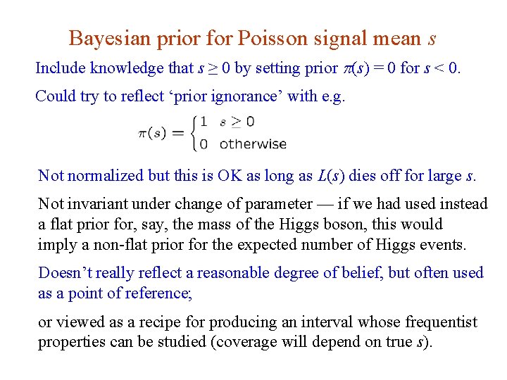
Bayesian prior for Poisson signal mean s Include knowledge that s ≥ 0 by setting prior p(s) = 0 for s < 0. Could try to reflect ‘prior ignorance’ with e. g. Not normalized but this is OK as long as L(s) dies off for large s. Not invariant under change of parameter — if we had used instead a flat prior for, say, the mass of the Higgs boson, this would imply a non-flat prior for the expected number of Higgs events. Doesn’t really reflect a reasonable degree of belief, but often used as a point of reference; or viewed as a recipe for producing an interval whose frequentist properties can be studied (coverage will depend on true s). G. Cowan Aachen 2014 / Statistics for Particle Physics, Lecture 4 18

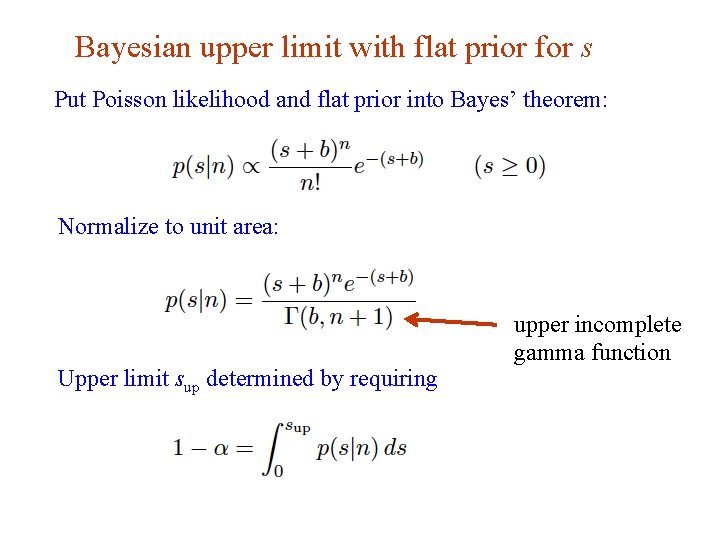
Bayesian upper limit with flat prior for s Put Poisson likelihood and flat prior into Bayes’ theorem: Normalize to unit area: Upper limit sup determined by requiring G. Cowan Aachen 2014 / Statistics for Particle Physics, Lecture 4 upper incomplete gamma function 19

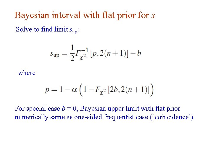
Bayesian interval with flat prior for s Solve to find limit sup: where For special case b = 0, Bayesian upper limit with flat prior numerically same as one-sided frequentist case (‘coincidence’). G. Cowan Aachen 2014 / Statistics for Particle Physics, Lecture 4 20

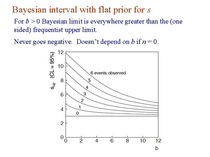
Bayesian interval with flat prior for s For b > 0 Bayesian limit is everywhere greater than the (one sided) frequentist upper limit. Never goes negative. Doesn’t depend on b if n = 0. G. Cowan Aachen 2014 / Statistics for Particle Physics, Lecture 4 21

Priors from formal rules Because of difficulties in encoding a vague degree of belief in a prior, one often attempts to derive the prior from formal rules, e. g. , to satisfy certain invariance principles or to provide maximum information gain for a certain set of measurements. Often called “objective priors” Form basis of Objective Bayesian Statistics The priors do not reflect a degree of belief (but might represent possible extreme cases). In Objective Bayesian analysis, can use the intervals in a frequentist way, i. e. , regard Bayes’ theorem as a recipe to produce an interval with certain coverage properties. G. Cowan Aachen 2014 / Statistics for Particle Physics, Lecture 4 22

Priors from formal rules (cont. ) For a review of priors obtained by formal rules see, e. g. , Formal priors have not been widely used in HEP, but there is recent interest in this direction, especially the reference priors of Bernardo and Berger; see e. g. L. Demortier, S. Jain and H. Prosper, Reference priors for high energy physics, Phys. Rev. D 82 (2010) 034002, ar. Xiv: 1002. 1111. D. Casadei, Reference analysis of the signal + background model in counting experiments, JINST 7 (2012) 01012; ar. Xiv: 1108. 4270. G. Cowan Aachen 2014 / Statistics for Particle Physics, Lecture 4 23

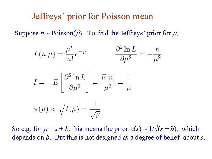
Jeffreys’ prior According to Jeffreys’ rule, take prior according to where is the Fisher information matrix. One can show that this leads to inference that is invariant under a transformation of parameters. For a Gaussian mean, the Jeffreys’ prior is constant; for a Poisson mean m it is proportional to 1/√m. G. Cowan Aachen 2014 / Statistics for Particle Physics, Lecture 4 24

Jeffreys’ prior for Poisson mean Suppose n ~ Poisson(m). To find the Jeffreys’ prior for m, So e. g. for m = s + b, this means the prior p(s) ~ 1/√(s + b), which depends on b. But this is not designed as a degree of belief about s. G. Cowan Aachen 2014 / Statistics for Particle Physics, Lecture 4 25

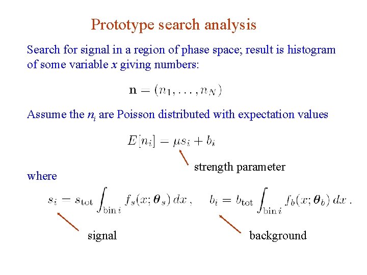
Prototype search analysis Search for signal in a region of phase space; result is histogram of some variable x giving numbers: Assume the ni are Poisson distributed with expectation values strength parameter where signal G. Cowan Aachen 2014 / Statistics for Particle Physics, Lecture 4 background 26

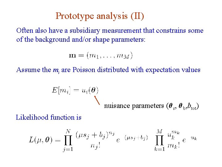
Prototype analysis (II) Often also have a subsidiary measurement that constrains some of the background and/or shape parameters: Assume the mi are Poisson distributed with expectation values nuisance parameters (θ s, θ b, btot) Likelihood function is G. Cowan Aachen 2014 / Statistics for Particle Physics, Lecture 4 27

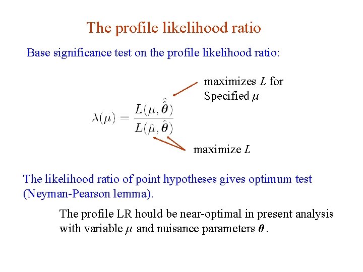
The profile likelihood ratio Base significance test on the profile likelihood ratio: maximizes L for Specified μ maximize L The likelihood ratio of point hypotheses gives optimum test (Neyman-Pearson lemma). The profile LR hould be near-optimal in present analysis with variable μ and nuisance parameters θ. G. Cowan Aachen 2014 / Statistics for Particle Physics, Lecture 4 28

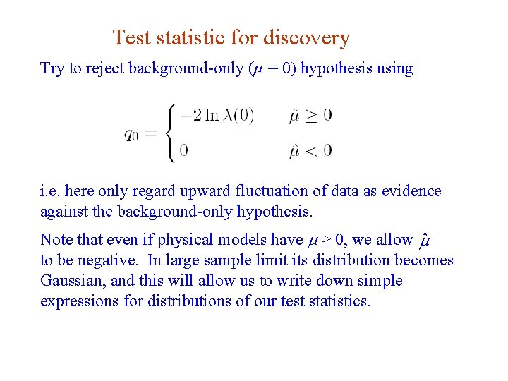
Test statistic for discovery Try to reject background-only (μ = 0) hypothesis using i. e. here only regard upward fluctuation of data as evidence against the background-only hypothesis. Note that even if physical models have m ≥ 0, we allow to be negative. In large sample limit its distribution becomes Gaussian, and this will allow us to write down simple expressions for distributions of our test statistics. G. Cowan Aachen 2014 / Statistics for Particle Physics, Lecture 4 29

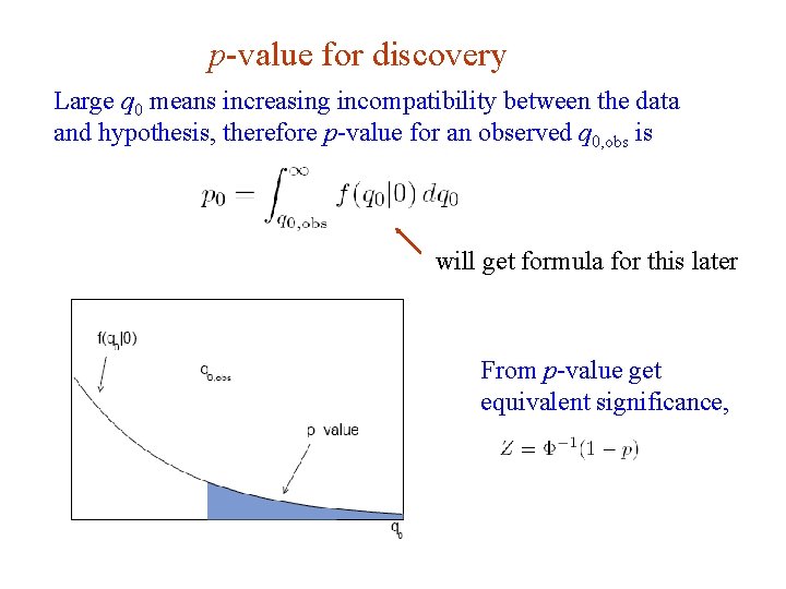
p-value for discovery Large q 0 means increasing incompatibility between the data and hypothesis, therefore p-value for an observed q 0, obs is will get formula for this later From p-value get equivalent significance, G. Cowan Aachen 2014 / Statistics for Particle Physics, Lecture 4 30

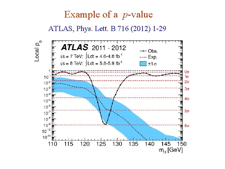
Example of a p-value ATLAS, Phys. Lett. B 716 (2012) 1 -29 G. Cowan Aachen 2014 / Statistics for Particle Physics, Lecture 4 31

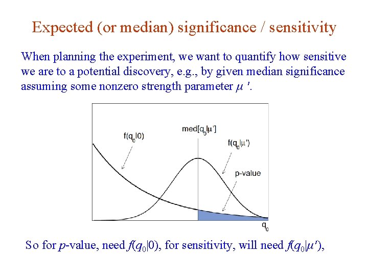
Expected (or median) significance / sensitivity When planning the experiment, we want to quantify how sensitive we are to a potential discovery, e. g. , by given median significance assuming some nonzero strength parameter μ ′. So for p-value, need f(q 0|0), for sensitivity, will need f(q 0|μ′), G. Cowan Aachen 2014 / Statistics for Particle Physics, Lecture 4 32

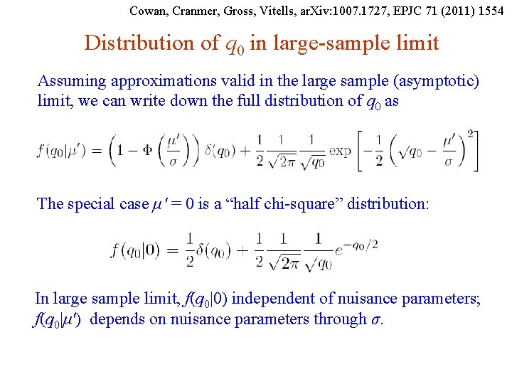
Cowan, Cranmer, Gross, Vitells, ar. Xiv: 1007. 1727, EPJC 71 (2011) 1554 Distribution of q 0 in large-sample limit Assuming approximations valid in the large sample (asymptotic) limit, we can write down the full distribution of q 0 as The special case μ′ = 0 is a “half chi-square” distribution: In large sample limit, f(q 0|0) independent of nuisance parameters; f(q 0|μ′) depends on nuisance parameters through σ. G. Cowan Aachen 2014 / Statistics for Particle Physics, Lecture 4 33

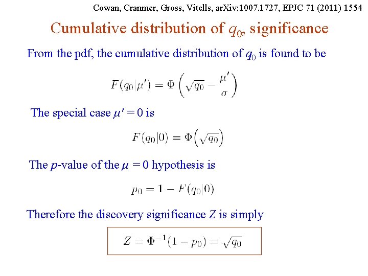
Cowan, Cranmer, Gross, Vitells, ar. Xiv: 1007. 1727, EPJC 71 (2011) 1554 Cumulative distribution of q 0, significance From the pdf, the cumulative distribution of q 0 is found to be The special case μ′ = 0 is The p-value of the μ = 0 hypothesis is Therefore the discovery significance Z is simply G. Cowan Aachen 2014 / Statistics for Particle Physics, Lecture 4 34

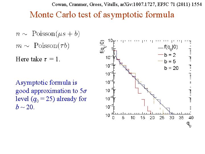
Cowan, Cranmer, Gross, Vitells, ar. Xiv: 1007. 1727, EPJC 71 (2011) 1554 Monte Carlo test of asymptotic formula Here take τ = 1. Asymptotic formula is good approximation to 5σ level (q 0 = 25) already for b ~ 20. G. Cowan Aachen 2014 / Statistics for Particle Physics, Lecture 4 35

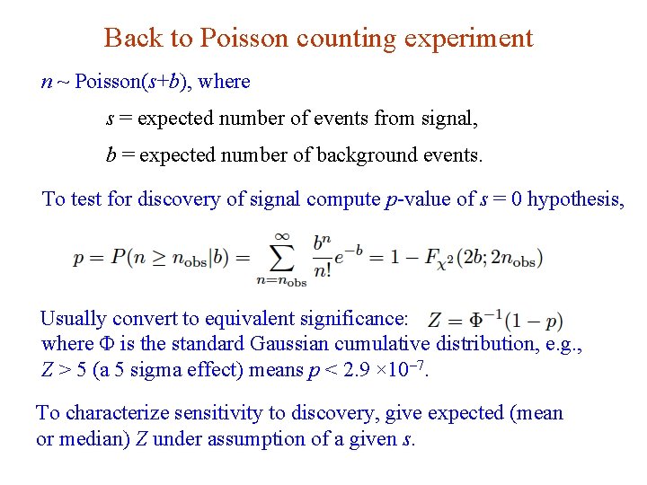
Back to Poisson counting experiment n ~ Poisson(s+b), where s = expected number of events from signal, b = expected number of background events. To test for discovery of signal compute p-value of s = 0 hypothesis, Usually convert to equivalent significance: where Φ is the standard Gaussian cumulative distribution, e. g. , Z > 5 (a 5 sigma effect) means p < 2. 9 × 10 -7. To characterize sensitivity to discovery, give expected (mean or median) Z under assumption of a given s. G. Cowan Aachen 2014 / Statistics for Particle Physics, Lecture 4 36

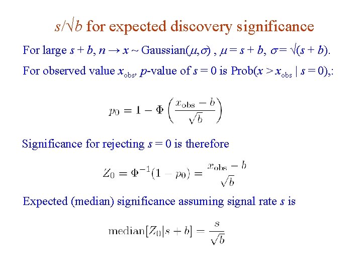
s/√b for expected discovery significance For large s + b, n → x ~ Gaussian(m, s) , m = s + b, s = √(s + b). For observed value xobs, p-value of s = 0 is Prob(x > xobs | s = 0), : Significance for rejecting s = 0 is therefore Expected (median) significance assuming signal rate s is G. Cowan Aachen 2014 / Statistics for Particle Physics, Lecture 4 37

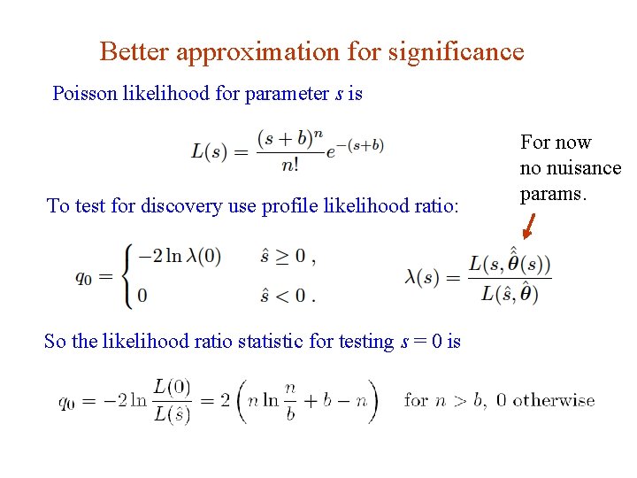
Better approximation for significance Poisson likelihood for parameter s is To test for discovery use profile likelihood ratio: For now no nuisance params. So the likelihood ratio statistic for testing s = 0 is G. Cowan Aachen 2014 / Statistics for Particle Physics, Lecture 4 38

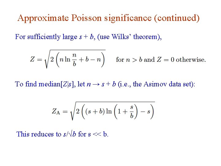
Approximate Poisson significance (continued) For sufficiently large s + b, (use Wilks’ theorem), To find median[Z|s], let n → s + b (i. e. , the Asimov data set): This reduces to s/√b for s << b. G. Cowan Aachen 2014 / Statistics for Particle Physics, Lecture 4 39

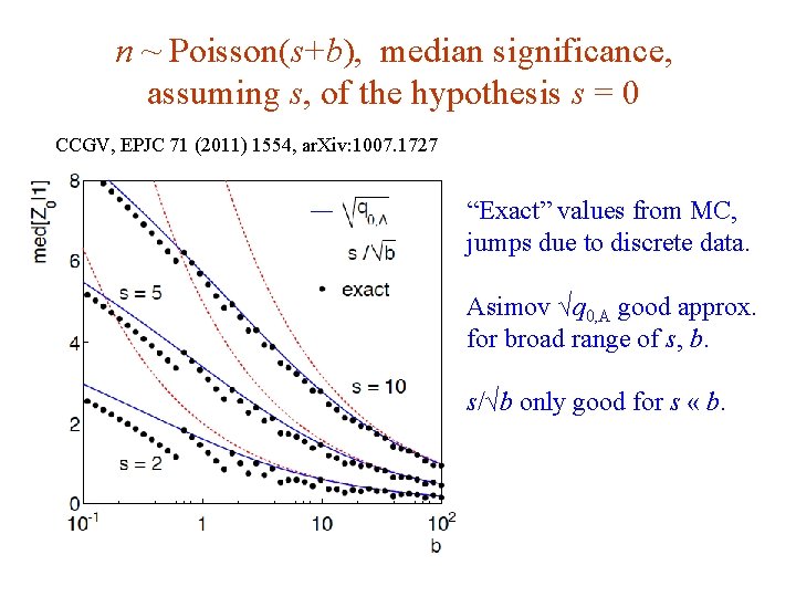
n ~ Poisson(s+b), median significance, assuming s, of the hypothesis s = 0 CCGV, EPJC 71 (2011) 1554, ar. Xiv: 1007. 1727 “Exact” values from MC, jumps due to discrete data. Asimov √q 0, A good approx. for broad range of s, b. s/√b only good for s « b. G. Cowan Aachen 2014 / Statistics for Particle Physics, Lecture 4 40

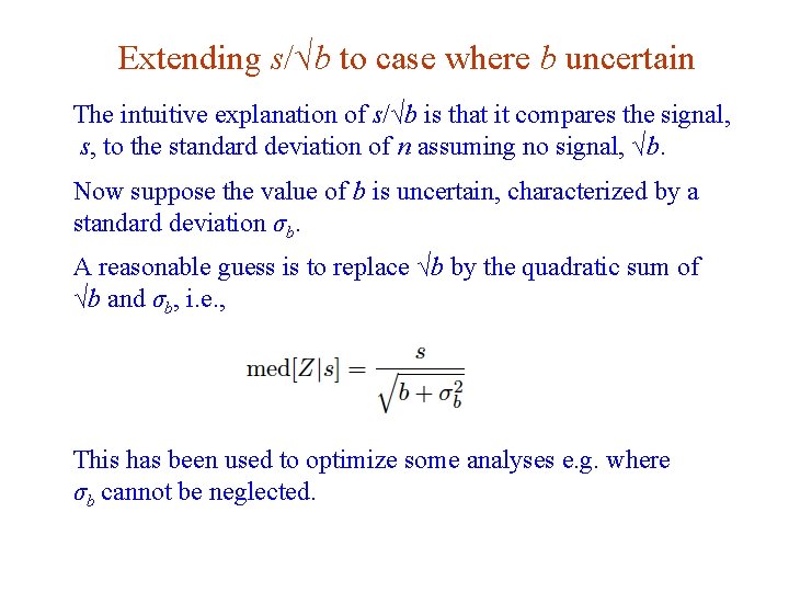
Extending s/√b to case where b uncertain The intuitive explanation of s/√b is that it compares the signal, s, to the standard deviation of n assuming no signal, √b. Now suppose the value of b is uncertain, characterized by a standard deviation σb. A reasonable guess is to replace √b by the quadratic sum of √b and σb, i. e. , This has been used to optimize some analyses e. g. where σb cannot be neglected. G. Cowan Aachen 2014 / Statistics for Particle Physics, Lecture 4 41

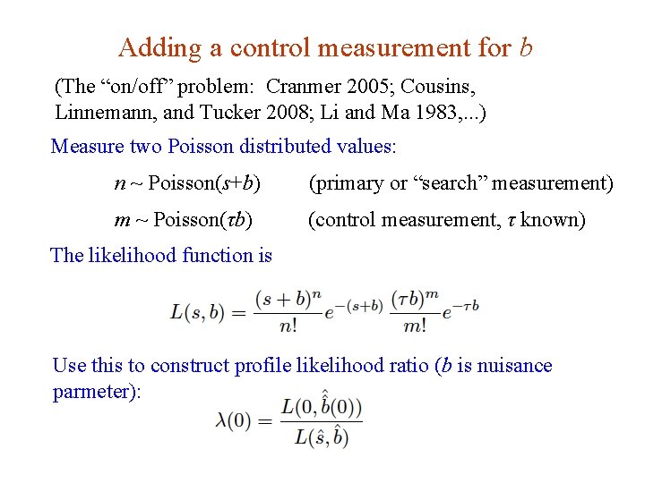
Adding a control measurement for b (The “on/off” problem: Cranmer 2005; Cousins, Linnemann, and Tucker 2008; Li and Ma 1983, . . . ) Measure two Poisson distributed values: n ~ Poisson(s+b) (primary or “search” measurement) m ~ Poisson(τb) (control measurement, τ known) The likelihood function is Use this to construct profile likelihood ratio (b is nuisance parmeter): G. Cowan Aachen 2014 / Statistics for Particle Physics, Lecture 4 42

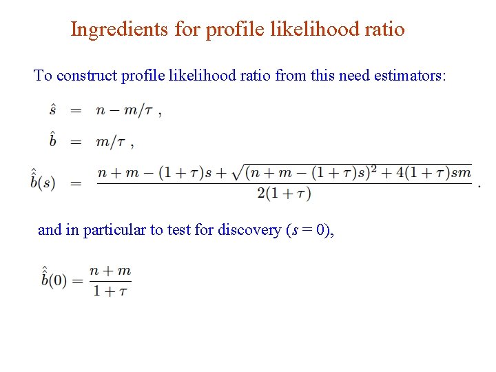
Ingredients for profile likelihood ratio To construct profile likelihood ratio from this need estimators: and in particular to test for discovery (s = 0), G. Cowan Aachen 2014 / Statistics for Particle Physics, Lecture 4 43

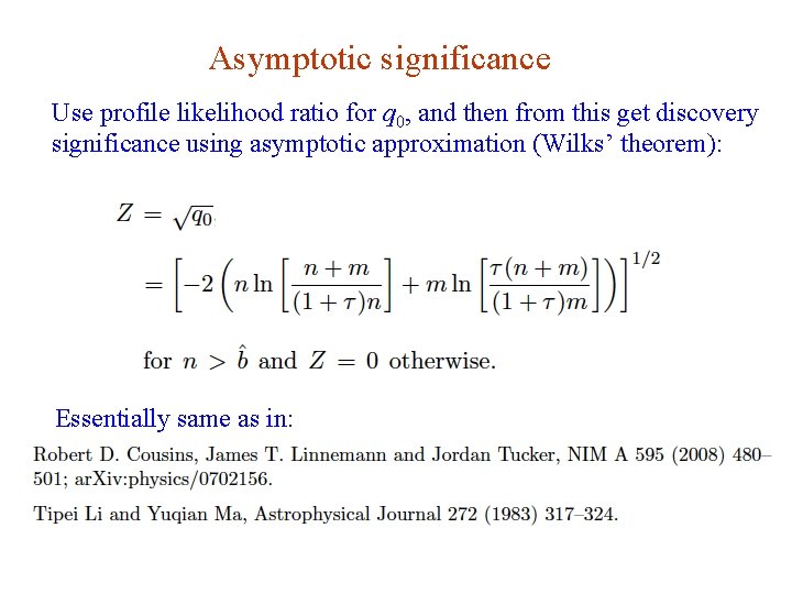
Asymptotic significance Use profile likelihood ratio for q 0, and then from this get discovery significance using asymptotic approximation (Wilks’ theorem): Essentially same as in: G. Cowan Aachen 2014 / Statistics for Particle Physics, Lecture 4 44

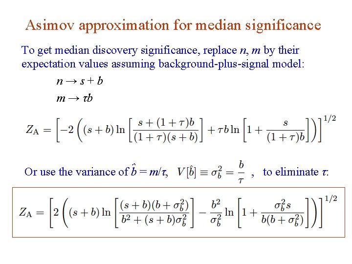
Asimov approximation for median significance To get median discovery significance, replace n, m by their expectation values assuming background-plus-signal model: n→s+b m → τb Or use the variance of ˆb = m/τ, G. Cowan Aachen 2014 / Statistics for Particle Physics, Lecture 4 , to eliminate τ: 45

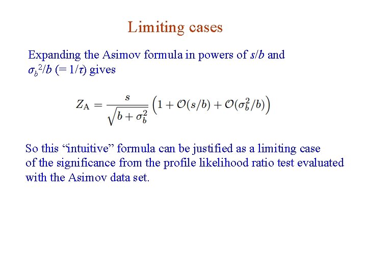
Limiting cases Expanding the Asimov formula in powers of s/b and σb 2/b (= 1/τ) gives So this “intuitive” formula can be justified as a limiting case of the significance from the profile likelihood ratio test evaluated with the Asimov data set. G. Cowan Aachen 2014 / Statistics for Particle Physics, Lecture 4 46

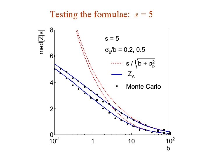
Testing the formulae: s = 5 G. Cowan Aachen 2014 / Statistics for Particle Physics, Lecture 4 47

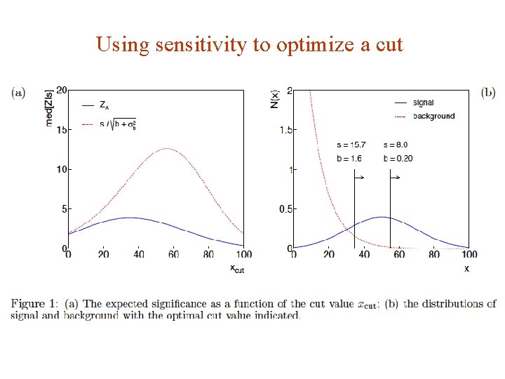
Using sensitivity to optimize a cut G. Cowan Aachen 2014 / Statistics for Particle Physics, Lecture 4 48

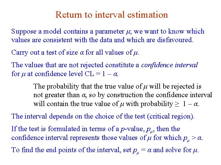
Return to interval estimation Suppose a model contains a parameter μ; we want to know which values are consistent with the data and which are disfavoured. Carry out a test of size α for all values of μ. The values that are not rejected constitute a confidence interval for μ at confidence level CL = 1 – α. The probability that the true value of μ will be rejected is not greater than α, so by construction the confidence interval will contain the true value of μ with probability ≥ 1 – α. The interval depends on the choice of the test (critical region). If the test is formulated in terms of a p-value, pμ, then the confidence interval represents those values of μ for which pμ > α. To find the end points of the interval, set pμ = α and solve for μ. G. Cowan Aachen 2014 / Statistics for Particle Physics, Lecture 4 49

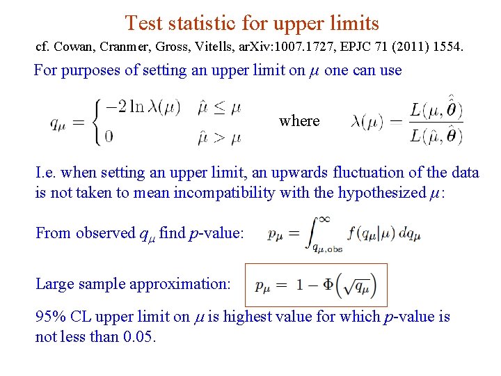
Test statistic for upper limits cf. Cowan, Cranmer, Gross, Vitells, ar. Xiv: 1007. 1727, EPJC 71 (2011) 1554. For purposes of setting an upper limit on μ one can use where I. e. when setting an upper limit, an upwards fluctuation of the data is not taken to mean incompatibility with the hypothesized μ: From observed qm find p-value: Large sample approximation: 95% CL upper limit on m is highest value for which p-value is not less than 0. 05. G. Cowan Aachen 2014 / Statistics for Particle Physics, Lecture 4 50

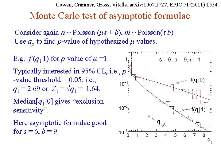
Cowan, Cranmer, Gross, Vitells, ar. Xiv: 1007. 1727, EPJC 71 (2011) 1554 Monte Carlo test of asymptotic formulae Consider again n ~ Poisson (μs + b), m ~ Poisson(τ b) Use qμ to find p-value of hypothesized μ values. E. g. f (q 1|1) for p-value of μ =1. Typically interested in 95% CL, i. e. , p -value threshold = 0. 05, i. e. , q 1 = 2. 69 or Z 1 = √q 1 = 1. 64. Median[q 1 |0] gives “exclusion sensitivity”. Here asymptotic formulae good for s = 6, b = 9. G. Cowan Aachen 2014 / Statistics for Particle Physics, Lecture 4 51

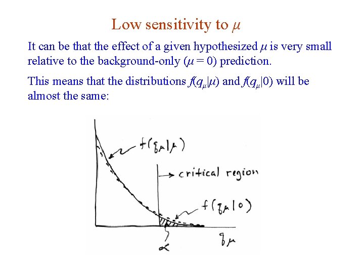
Low sensitivity to μ It can be that the effect of a given hypothesized μ is very small relative to the background-only (μ = 0) prediction. This means that the distributions f(qμ|μ) and f(qμ|0) will be almost the same: G. Cowan Aachen 2014 / Statistics for Particle Physics, Lecture 4 52

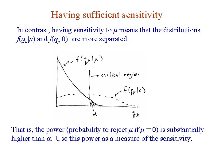
Having sufficient sensitivity In contrast, having sensitivity to μ means that the distributions f(qμ|μ) and f(qμ|0) are more separated: That is, the power (probability to reject μ if μ = 0) is substantially higher than α. Use this power as a measure of the sensitivity. G. Cowan Aachen 2014 / Statistics for Particle Physics, Lecture 4 53

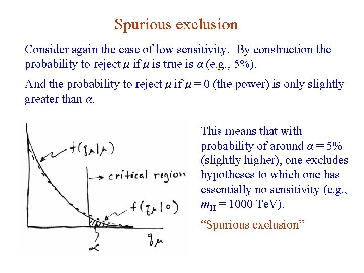
Spurious exclusion Consider again the case of low sensitivity. By construction the probability to reject μ if μ is true is α (e. g. , 5%). And the probability to reject μ if μ = 0 (the power) is only slightly greater than α. This means that with probability of around α = 5% (slightly higher), one excludes hypotheses to which one has essentially no sensitivity (e. g. , m. H = 1000 Te. V). “Spurious exclusion” G. Cowan Aachen 2014 / Statistics for Particle Physics, Lecture 4 54

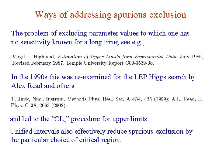
Ways of addressing spurious exclusion The problem of excluding parameter values to which one has no sensitivity known for a long time; see e. g. , In the 1990 s this was re-examined for the LEP Higgs search by Alex Read and others and led to the “CLs” procedure for upper limits. Unified intervals also effectively reduce spurious exclusion by the particular choice of critical region. G. Cowan Aachen 2014 / Statistics for Particle Physics, Lecture 4 55

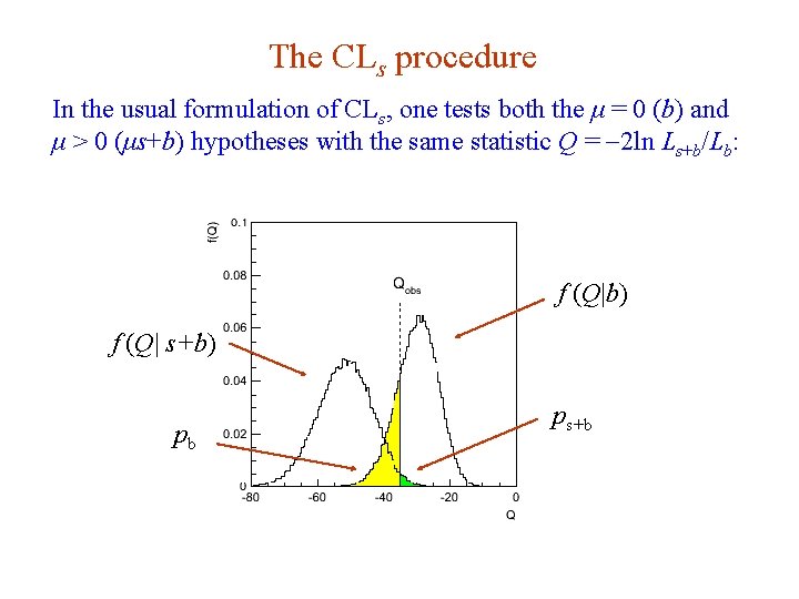
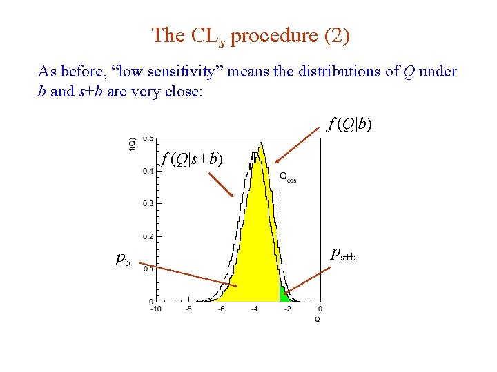
The CLs procedure In the usual formulation of CLs, one tests both the μ = 0 (b) and μ > 0 (μs+b) hypotheses with the same statistic Q = -2 ln Ls+b/Lb: f (Q|b) f (Q| s+b) pb G. Cowan Aachen 2014 / Statistics for Particle Physics, Lecture 4 ps+b 56

The CLs procedure (2) As before, “low sensitivity” means the distributions of Q under b and s+b are very close: f (Q|b) f (Q|s+b) pb G. Cowan Aachen 2014 / Statistics for Particle Physics, Lecture 4 ps+b 57

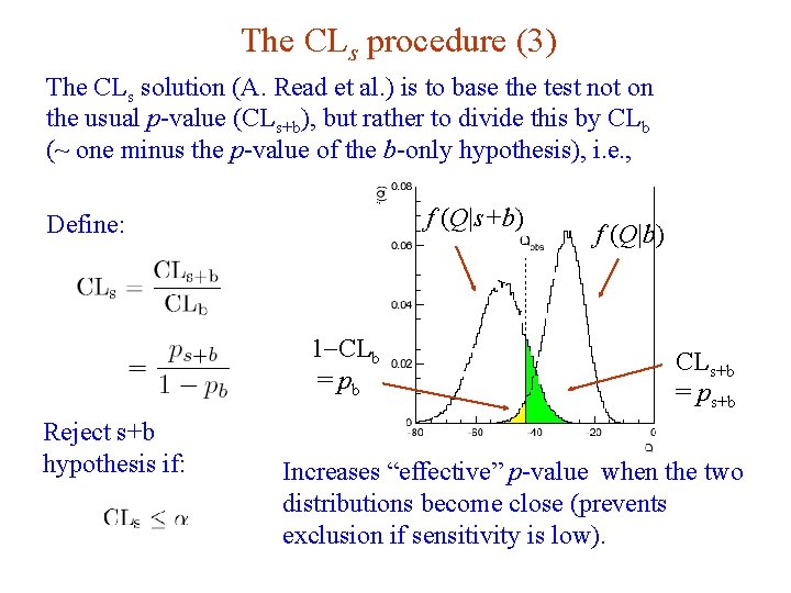
The CLs procedure (3) The CLs solution (A. Read et al. ) is to base the test not on the usual p-value (CLs+b), but rather to divide this by CLb (~ one minus the p-value of the b-only hypothesis), i. e. , f (Q|s+b) Define: 1 -CLb = pb Reject s+b hypothesis if: G. Cowan f (Q|b) CLs+b = ps+b Increases “effective” p-value when the two distributions become close (prevents exclusion if sensitivity is low). Aachen 2014 / Statistics for Particle Physics, Lecture 4 58

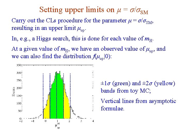
Setting upper limits on μ = σ/σSM Carry out the CLs procedure for the parameter μ = σ/σSM, resulting in an upper limit μup. In, e. g. , a Higgs search, this is done for each value of m. H. At a given value of m. H, we have an observed value of μup, and we can also find the distribution f(μup|0): ± 1σ (green) and ± 2σ (yellow) bands from toy MC; Vertical lines from asymptotic formulae. G. Cowan Aachen 2014 / Statistics for Particle Physics, Lecture 4 59

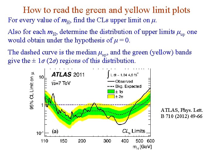
How to read the green and yellow limit plots For every value of m. H, find the CLs upper limit on μ. Also for each m. H, determine the distribution of upper limits μup one would obtain under the hypothesis of μ = 0. The dashed curve is the median μup, and the green (yellow) bands give the ± 1σ (2σ) regions of this distribution. ATLAS, Phys. Lett. B 710 (2012) 49 -66 G. Cowan Aachen 2014 / Statistics for Particle Physics, Lecture 4 60

Choice of test for limits (2) In some cases μ = 0 is no longer a relevant alternative and we want to try to exclude μ on the grounds that some other measure of incompatibility between it and the data exceeds some threshold. If the measure of incompatibility is taken to be the likelihood ratio with respect to a two-sided alternative, then the critical region can contain both high and low data values. → unified intervals, G. Feldman, R. Cousins, Phys. Rev. D 57, 3873– 3889 (1998) The Big Debate is whether to use one-sided or unified intervals in cases where small (or zero) values of the parameter are relevant alternatives. Professional statisticians have voiced support on both sides of the debate. G. Cowan Aachen 2014 / Statistics for Particle Physics, Lecture 4 61

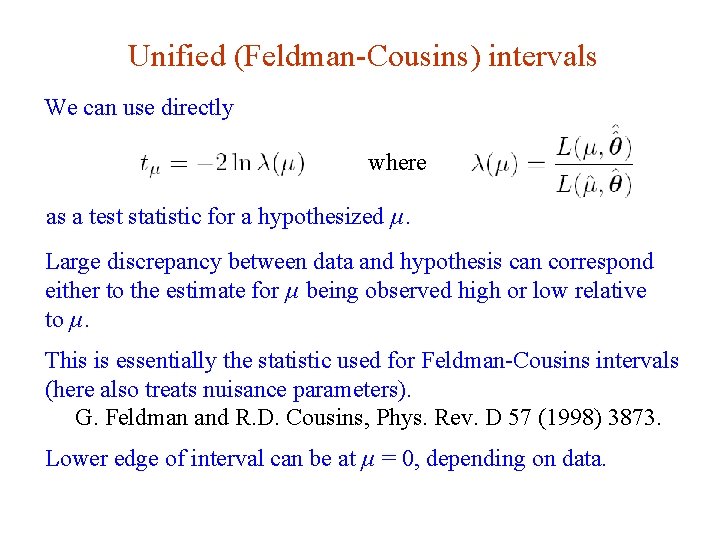
Unified (Feldman-Cousins) intervals We can use directly where as a test statistic for a hypothesized μ. Large discrepancy between data and hypothesis can correspond either to the estimate for μ being observed high or low relative to μ. This is essentially the statistic used for Feldman-Cousins intervals (here also treats nuisance parameters). G. Feldman and R. D. Cousins, Phys. Rev. D 57 (1998) 3873. Lower edge of interval can be at μ = 0, depending on data. G. Cowan Aachen 2014 / Statistics for Particle Physics, Lecture 4 62

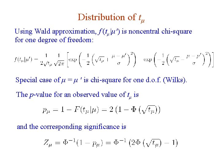
Distribution of tμ Using Wald approximation, f (tμ |μ′) is noncentral chi-square for one degree of freedom: Special case of μ = μ ′ is chi-square for one d. o. f. (Wilks). The p-value for an observed value of tμ is and the corresponding significance is G. Cowan Aachen 2014 / Statistics for Particle Physics, Lecture 4 63

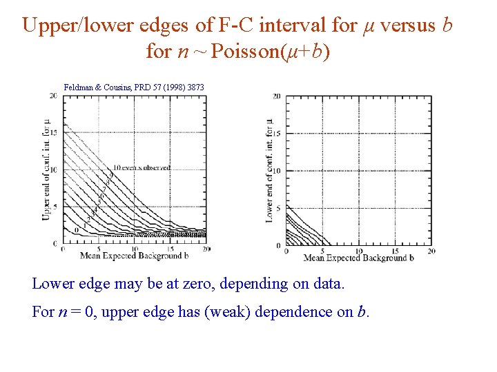
Upper/lower edges of F-C interval for μ versus b for n ~ Poisson(μ+b) Feldman & Cousins, PRD 57 (1998) 3873 Lower edge may be at zero, depending on data. For n = 0, upper edge has (weak) dependence on b. G. Cowan Aachen 2014 / Statistics for Particle Physics, Lecture 4 64

Feldman-Cousins discussion The initial motivation for Feldman-Cousins (unified) confidence intervals was to eliminate null intervals. The F-C limits are based on a likelihood ratio for a test of μ with respect to the alternative consisting of all other allowed values of μ (not just, say, lower values). The interval’s upper edge is higher than the limit from the onesided test, and lower values of μ may be excluded as well. A substantial downward fluctuation in the data gives a low (but nonzero) limit. This means that when a value of μ is excluded, it is because there is a probability α for the data to fluctuate either high or low in a manner corresponding to less compatibility as measured by the likelihood ratio. G. Cowan Cargese 2012 / Statistics for HEP / Lecture 2 65