Statistical Methods for Particle Physics Lecture 2 multivariate

Statistical Methods for Particle Physics Lecture 2: multivariate methods https: //indico. cern. ch/event/738002/ IX NEx. T Ph. D Workshop: Decoding New Physics Cosener’s House, Abingdon 8 -11 July 2019 Glen Cowan Physics Department Royal Holloway, University of London g. cowan@rhul. ac. uk www. pp. rhul. ac. uk/~cowan G. Cowan NEx. T Workshop, 2019 / GDC Lecture 2 1

Outline Lecture 1: Introduction and review of fundamentals Review of probability Parameter estimation, maximum likelihood Statistical tests for discovery and limits Lecture 2: Multivariate methods Neyman-Pearson lemma Fisher discriminant, neural networks Boosted decision trees Lecture 3: Further topics Nuisance parameters (Bayesian and frequentist) Experimental sensitivity Revisiting limits G. Cowan NEx. T Workshop, 2019 / GDC Lecture 2 2

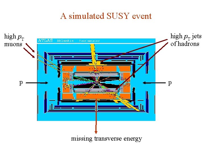
A simulated SUSY event high p. T jets of hadrons high p. T muons p p missing transverse energy G. Cowan NEx. T Workshop, 2019 / GDC Lecture 2 3

Background events This event from Standard Model ttbar production also has high p. T jets and muons, and some missing transverse energy. → can easily mimic a SUSY event. G. Cowan NEx. T Workshop, 2019 / GDC Lecture 2 4

Physics context of a statistical test Event Selection: the event types in question are both known to exist. Example: separation of different particle types (electron vs muon) or known event types (ttbar vs QCD multijet). E. g. test H 0 : event is background vs. H 1 : event is signal. Use selected events for further study. Search for New Physics: the null hypothesis is H 0 : all events correspond to Standard Model (background only), and the alternative is H 1 : events include a type whose existence is not yet established (signal plus background) Many subtle issues here, mainly related to the high standard of proof required to establish presence of a new phenomenon. The optimal statistical test for a search is closely related to that used for event selection. G. Cowan NEx. T Workshop, 2019 / GDC Lecture 2 5

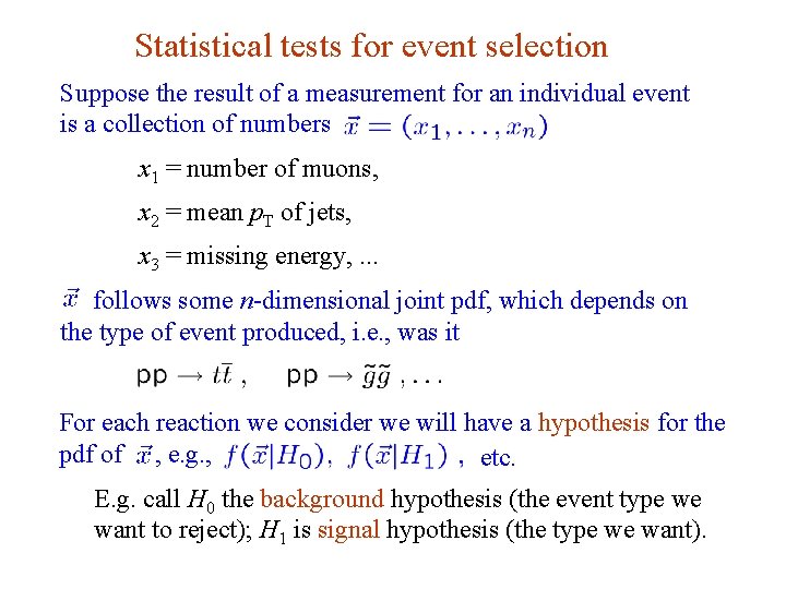
Statistical tests for event selection Suppose the result of a measurement for an individual event is a collection of numbers x 1 = number of muons, x 2 = mean p. T of jets, x 3 = missing energy, . . . follows some n-dimensional joint pdf, which depends on the type of event produced, i. e. , was it For each reaction we consider we will have a hypothesis for the pdf of , e. g. , etc. E. g. call H 0 the background hypothesis (the event type we want to reject); H 1 is signal hypothesis (the type we want). G. Cowan NEx. T Workshop, 2019 / GDC Lecture 2 6

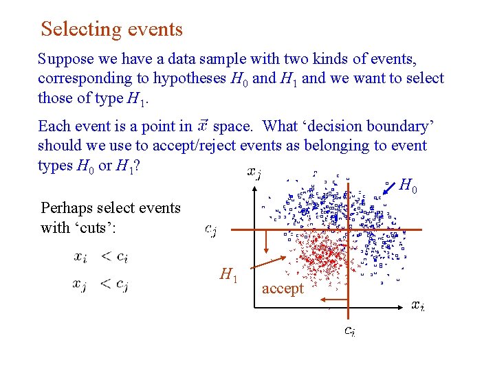
Selecting events Suppose we have a data sample with two kinds of events, corresponding to hypotheses H 0 and H 1 and we want to select those of type H 1. Each event is a point in space. What ‘decision boundary’ should we use to accept/reject events as belonging to event types H 0 or H 1? H 0 Perhaps select events with ‘cuts’: H 1 G. Cowan accept NEx. T Workshop, 2019 / GDC Lecture 2 7

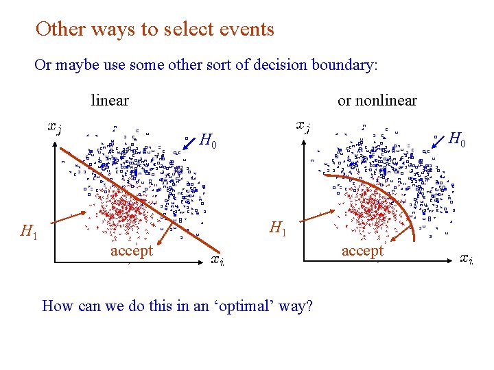
Other ways to select events Or maybe use some other sort of decision boundary: linear or nonlinear H 0 H 1 accept How can we do this in an ‘optimal’ way? G. Cowan NEx. T Workshop, 2019 / GDC Lecture 2 8

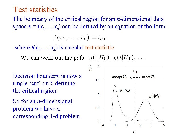
Test statistics The boundary of the critical region for an n-dimensional data space x = (x 1, . . . , xn) can be defined by an equation of the form where t(x 1, …, xn) is a scalar test statistic. We can work out the pdfs Decision boundary is now a single ‘cut’ on t, defining the critical region. So for an n-dimensional problem we have a corresponding 1 -d problem. G. Cowan NEx. T Workshop, 2019 / GDC Lecture 2 9

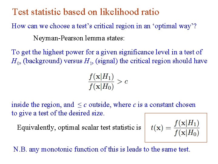
Test statistic based on likelihood ratio How can we choose a test’s critical region in an ‘optimal way’? Neyman-Pearson lemma states: To get the highest power for a given significance level in a test of H 0, (background) versus H 1, (signal) the critical region should have inside the region, and ≤ c outside, where c is a constant chosen to give a test of the desired size. Equivalently, optimal scalar test statistic is N. B. any monotonic function of this is leads to the same test. G. Cowan NEx. T Workshop, 2019 / GDC Lecture 2 10

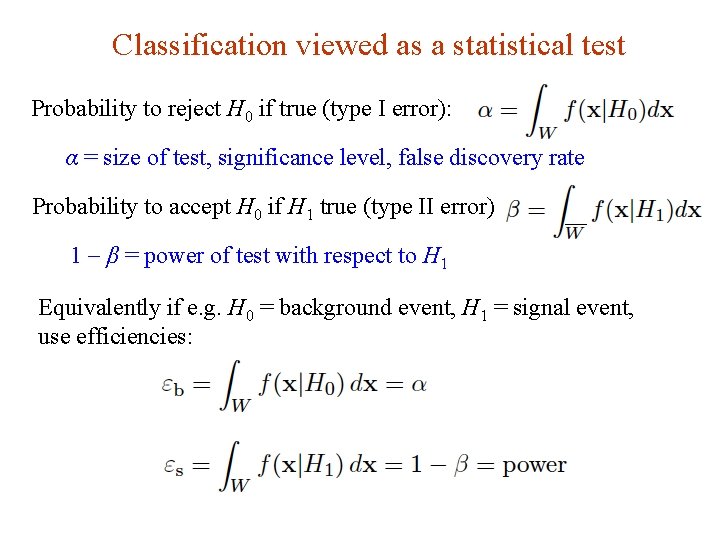
Classification viewed as a statistical test Probability to reject H 0 if true (type I error): α = size of test, significance level, false discovery rate Probability to accept H 0 if H 1 true (type II error): 1 - β = power of test with respect to H 1 Equivalently if e. g. H 0 = background event, H 1 = signal event, use efficiencies: G. Cowan NEx. T Workshop, 2019 / GDC Lecture 2 11

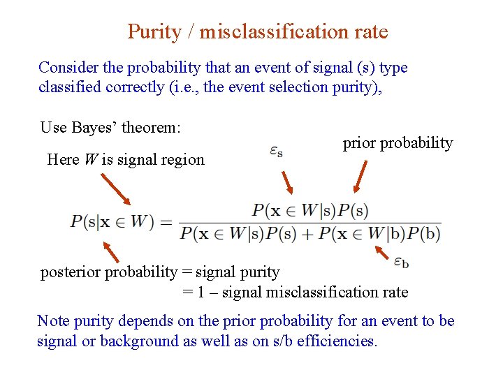
Purity / misclassification rate Consider the probability that an event of signal (s) type classified correctly (i. e. , the event selection purity), Use Bayes’ theorem: Here W is signal region prior probability posterior probability = signal purity = 1 – signal misclassification rate Note purity depends on the prior probability for an event to be signal or background as well as on s/b efficiencies. G. Cowan NEx. T Workshop, 2019 / GDC Lecture 2 12

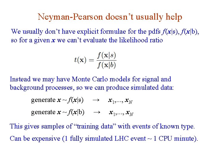
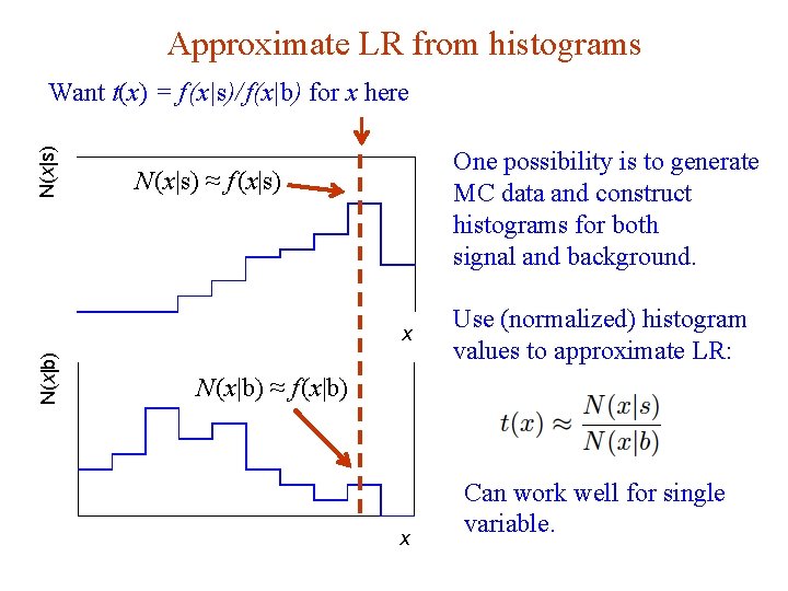
Neyman-Pearson doesn’t usually help We usually don’t have explicit formulae for the pdfs f (x|s), f (x|b), so for a given x we can’t evaluate the likelihood ratio Instead we may have Monte Carlo models for signal and background processes, so we can produce simulated data: generate x ~ f (x|s) → x 1, . . . , x. N generate x ~ f (x|b) → x 1, . . . , x. N This gives samples of “training data” with events of known type. Can be expensive (1 fully simulated LHC event ~ 1 CPU minute). G. Cowan NEx. T Workshop, 2019 / GDC Lecture 2 13

Approximate LR from histograms N(x|s) Want t(x) = f (x|s)/ f(x|b) for x here One possibility is to generate MC data and construct histograms for both signal and background. N (x|s) ≈ f (x|s) N(x|b) x N (x|b) ≈ f (x|b) x G. Cowan Use (normalized) histogram values to approximate LR: Can work well for single variable. NEx. T Workshop, 2019 / GDC Lecture 2 14

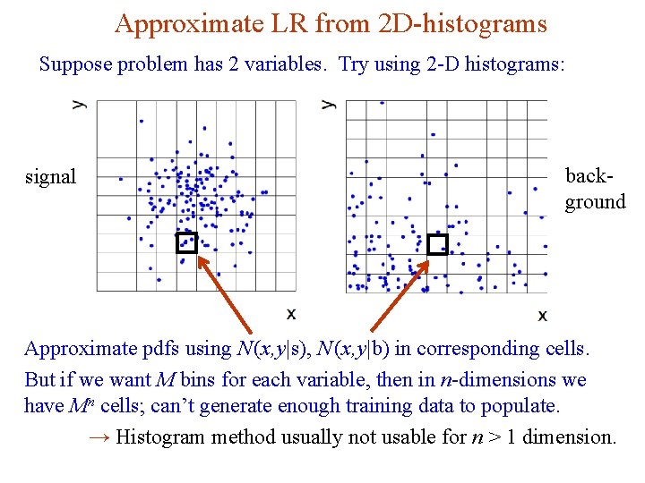
Approximate LR from 2 D-histograms Suppose problem has 2 variables. Try using 2 -D histograms: background signal Approximate pdfs using N (x, y|s), N (x, y|b) in corresponding cells. But if we want M bins for each variable, then in n-dimensions we have Mn cells; can’t generate enough training data to populate. → Histogram method usually not usable for n > 1 dimension. G. Cowan NEx. T Workshop, 2019 / GDC Lecture 2 15

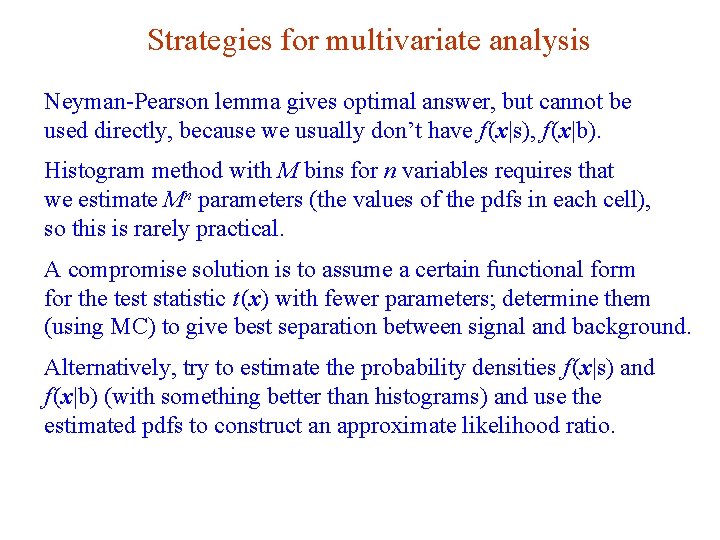
Strategies for multivariate analysis Neyman-Pearson lemma gives optimal answer, but cannot be used directly, because we usually don’t have f (x|s), f (x|b). Histogram method with M bins for n variables requires that we estimate Mn parameters (the values of the pdfs in each cell), so this is rarely practical. A compromise solution is to assume a certain functional form for the test statistic t (x) with fewer parameters; determine them (using MC) to give best separation between signal and background. Alternatively, try to estimate the probability densities f (x|s) and f (x|b) (with something better than histograms) and use the estimated pdfs to construct an approximate likelihood ratio. G. Cowan NEx. T Workshop, 2019 / GDC Lecture 2 16

Multivariate methods Many new (and some old) methods: Fisher discriminant (Deep) neural networks Kernel density methods Support Vector Machines Decision trees Boosting Bagging G. Cowan NEx. T Workshop, 2019 / GDC Lecture 2 17

Resources on multivariate methods C. M. Bishop, Pattern Recognition and Machine Learning, Springer, 2006 T. Hastie, R. Tibshirani, J. Friedman, The Elements of Statistical Learning, 2 nd ed. , Springer, 2009 R. Duda, P. Hart, D. Stork, Pattern Classification, 2 nd ed. , Wiley, 2001 A. Webb, Statistical Pattern Recognition, 2 nd ed. , Wiley, 2002. Ilya Narsky and Frank C. Porter, Statistical Analysis Techniques in Particle Physics, Wiley, 2014. 朱永生 （�著），��数据多元��分析， 科学出版社， 北 京，2009。 G. Cowan NEx. T Workshop, 2019 / GDC Lecture 2 18

Software Rapidly growing area of development – two important resources: TMVA, Höcker, Stelzer, Tegenfeldt, Voss, physics/0703039 From tmva. sourceforge. net, also distributed with ROOT Variety of classifiers Good manual, widely used in HEP scikit-learn Python-based tools for Machine Learning scikit-learn. org Large user community G. Cowan NEx. T Workshop, 2019 / GDC Lecture 2 19

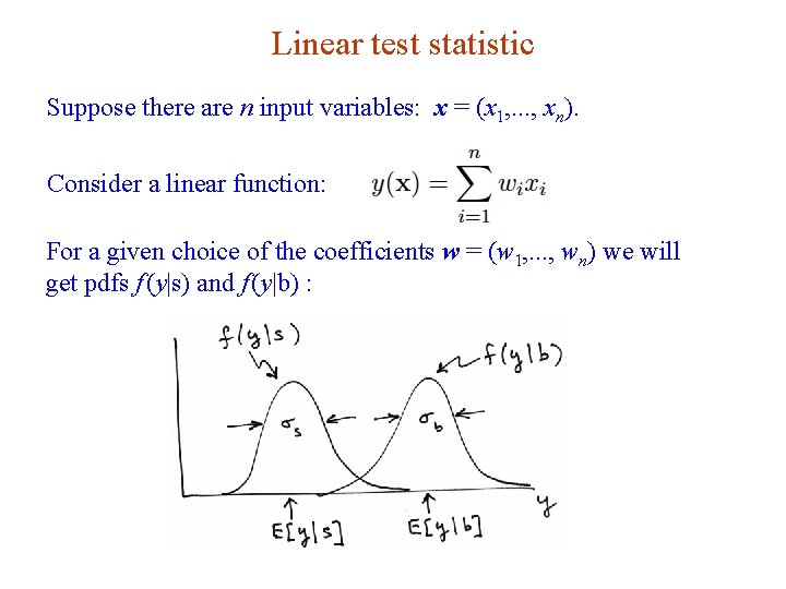
Linear test statistic Suppose there are n input variables: x = (x 1, . . . , xn). Consider a linear function: For a given choice of the coefficients w = (w 1, . . . , wn) we will get pdfs f (y|s) and f (y|b) : G. Cowan NEx. T Workshop, 2019 / GDC Lecture 2 20

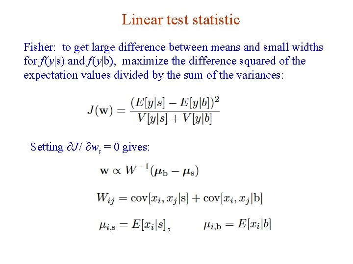
Linear test statistic Fisher: to get large difference between means and small widths for f (y|s) and f (y|b), maximize the difference squared of the expectation values divided by the sum of the variances: Setting ∂J / ∂wi = 0 gives: , G. Cowan NEx. T Workshop, 2019 / GDC Lecture 2 21

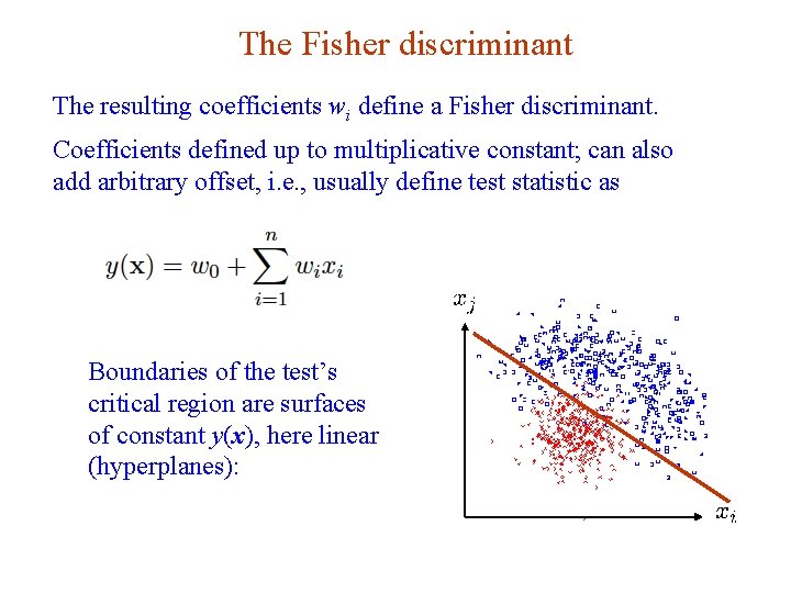
The Fisher discriminant The resulting coefficients wi define a Fisher discriminant. Coefficients defined up to multiplicative constant; can also add arbitrary offset, i. e. , usually define test statistic as Boundaries of the test’s critical region are surfaces of constant y(x), here linear (hyperplanes): G. Cowan NEx. T Workshop, 2019 / GDC Lecture 2 22

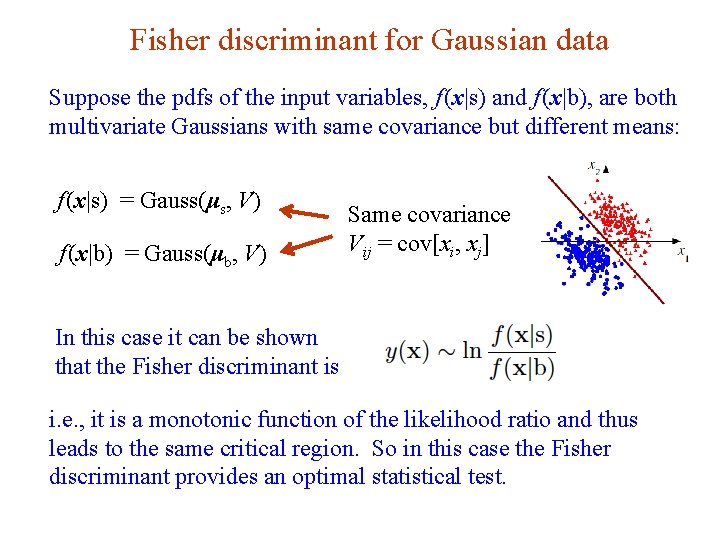
Fisher discriminant for Gaussian data Suppose the pdfs of the input variables, f (x|s) and f (x|b), are both multivariate Gaussians with same covariance but different means: f (x|s) = Gauss(μs, V) f (x|b) = Gauss(μb, V) Same covariance Vij = cov[xi, xj] In this case it can be shown that the Fisher discriminant is i. e. , it is a monotonic function of the likelihood ratio and thus leads to the same critical region. So in this case the Fisher discriminant provides an optimal statistical test. G. Cowan NEx. T Workshop, 2019 / GDC Lecture 2 23

G. Cowan NEx. T Workshop, 2019 / GDC Lecture 2 24

G. Cowan NEx. T Workshop, 2019 / GDC Lecture 2 25

G. Cowan NEx. T Workshop, 2019 / GDC Lecture 2 26

G. Cowan NEx. T Workshop, 2019 / GDC Lecture 2 27

G. Cowan NEx. T Workshop, 2019 / GDC Lecture 2 28

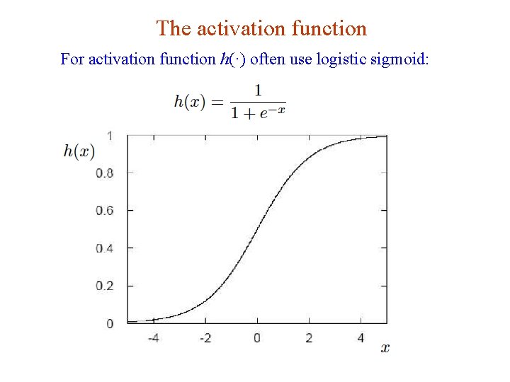
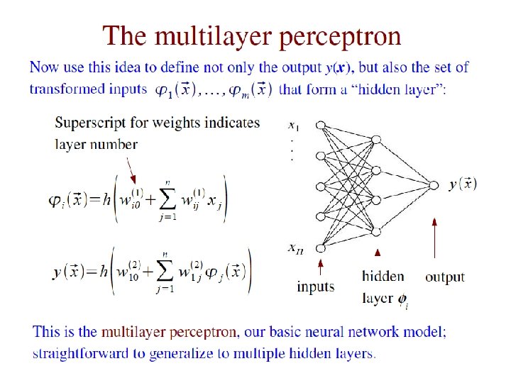
The activation function For activation function h(·) often use logistic sigmoid: G. Cowan NEx. T Workshop, 2019 / GDC Lecture 2 29

G. Cowan NEx. T Workshop, 2019 / GDC Lecture 2 30

G. Cowan NEx. T Workshop, 2019 / GDC Lecture 2 31

G. Cowan NEx. T Workshop, 2019 / GDC Lecture 2 32

G. Cowan NEx. T Workshop, 2019 / GDC Lecture 2 33

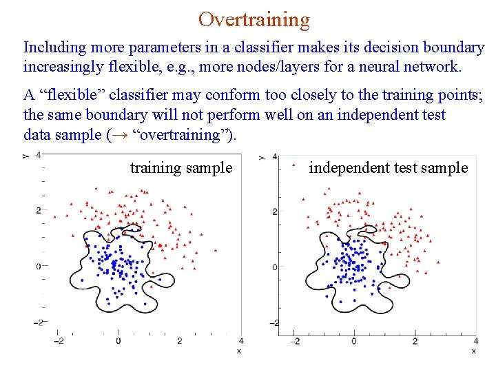
Overtraining Including more parameters in a classifier makes its decision boundary increasingly flexible, e. g. , more nodes/layers for a neural network. A “flexible” classifier may conform too closely to the training points; the same boundary will not perform well on an independent test data sample (→ “overtraining”). training sample G. Cowan independent test sample NEx. T Workshop, 2019 / GDC Lecture 2 34

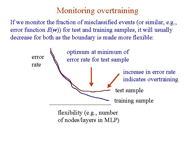
Monitoring overtraining If we monitor the fraction of misclassified events (or similar, e. g. , error function E(w)) for test and training samples, it will usually decrease for both as the boundary is made more flexible: error rate optimum at minimum of error rate for test sample increase in error rate indicates overtraining test sample training sample flexibility (e. g. , number of nodes/layers in MLP) G. Cowan NEx. T Workshop, 2019 / GDC Lecture 2 35

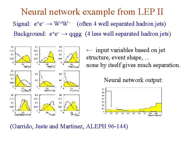
Neural network example from LEP II Signal: e+e- → W+W- (often 4 well separated hadron jets) Background: e+e- → qqgg (4 less well separated hadron jets) ← input variables based on jet structure, event shape, . . . none by itself gives much separation. Neural network output: (Garrido, Juste and Martinez, ALEPH 96 -144) G. Cowan NEx. T Workshop, 2019 / GDC Lecture 2 page 36

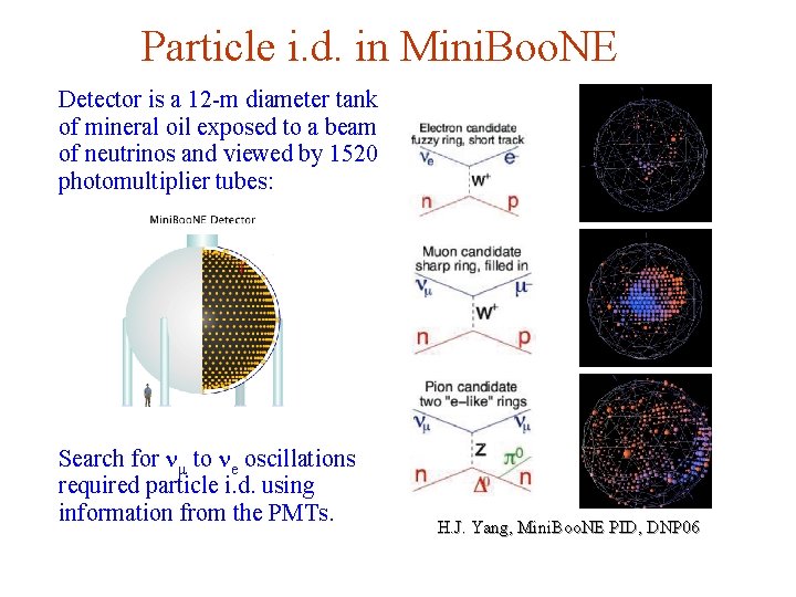
Particle i. d. in Mini. Boo. NE Detector is a 12 -m diameter tank of mineral oil exposed to a beam of neutrinos and viewed by 1520 photomultiplier tubes: Search for nm to ne oscillations required particle i. d. using information from the PMTs. G. Cowan H. J. Yang, Mini. Boo. NE PID, DNP 06 NEx. T Workshop, 2019 / GDC Lecture 2 page 37

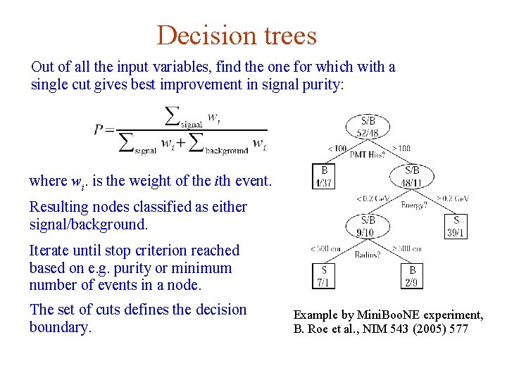
Decision trees Out of all the input variables, find the one for which with a single cut gives best improvement in signal purity: where wi. is the weight of the ith event. Resulting nodes classified as either signal/background. Iterate until stop criterion reached based on e. g. purity or minimum number of events in a node. The set of cuts defines the decision boundary. G. Cowan Example by Mini. Boo. NE experiment, B. Roe et al. , NIM 543 (2005) 577 NEx. T Workshop, 2019 / GDC Lecture 2 page 38

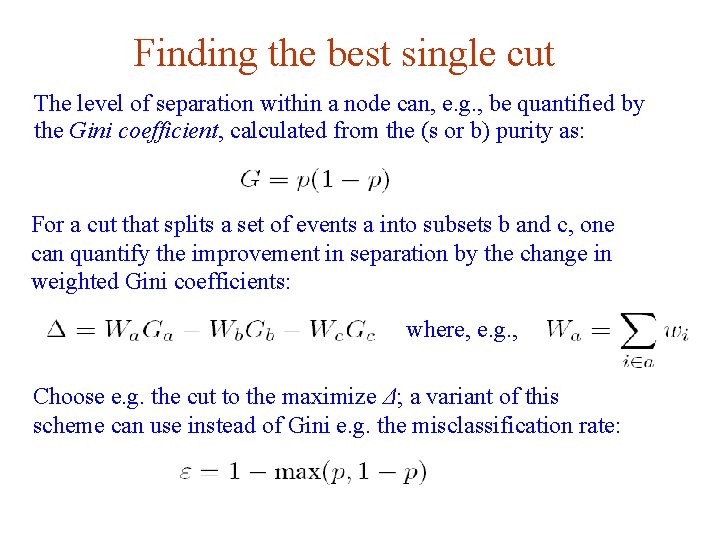
Finding the best single cut The level of separation within a node can, e. g. , be quantified by the Gini coefficient, calculated from the (s or b) purity as: For a cut that splits a set of events a into subsets b and c, one can quantify the improvement in separation by the change in weighted Gini coefficients: where, e. g. , Choose e. g. the cut to the maximize Δ; a variant of this scheme can use instead of Gini e. g. the misclassification rate: G. Cowan NEx. T Workshop, 2019 / GDC Lecture 2 page 39

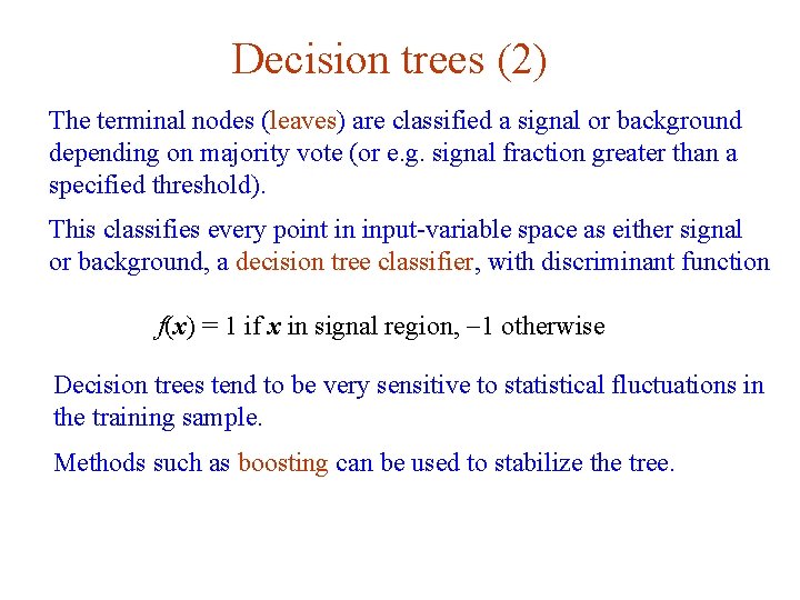
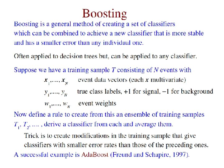
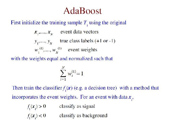
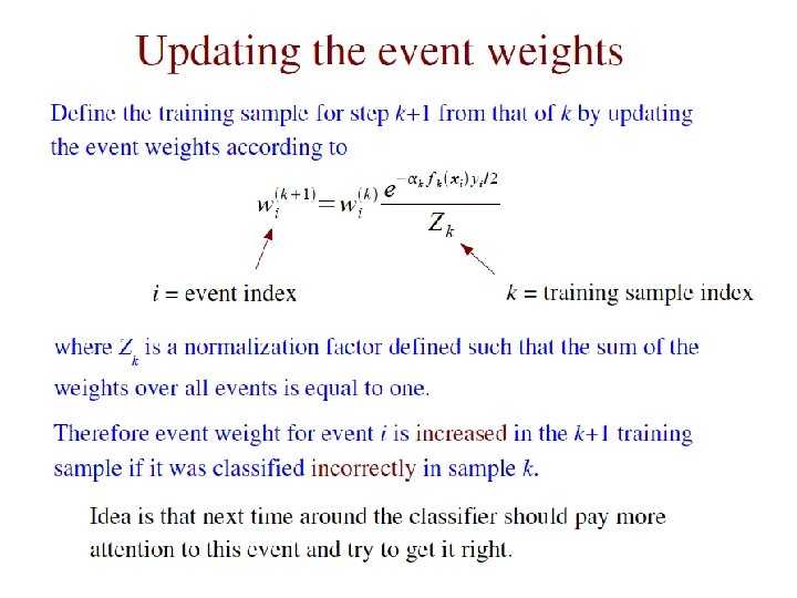
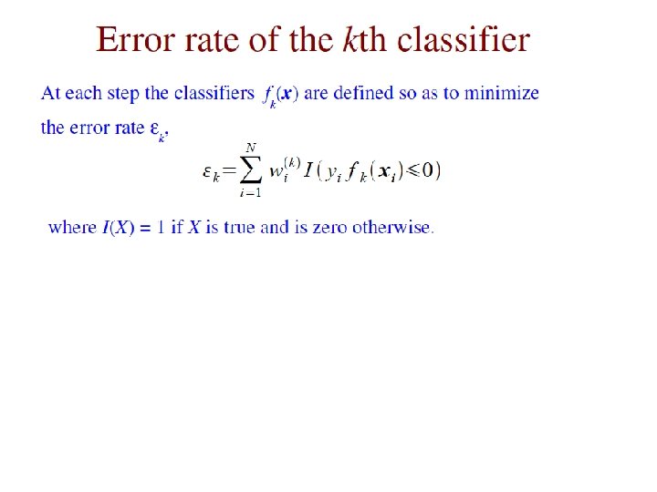
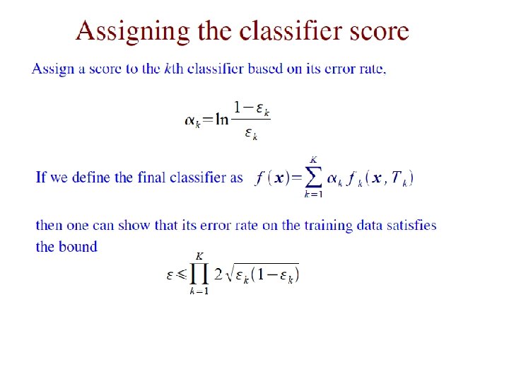
Decision trees (2) The terminal nodes (leaves) are classified a signal or background depending on majority vote (or e. g. signal fraction greater than a specified threshold). This classifies every point in input-variable space as either signal or background, a decision tree classifier, with discriminant function f(x) = 1 if x in signal region, -1 otherwise Decision trees tend to be very sensitive to statistical fluctuations in the training sample. Methods such as boosting can be used to stabilize the tree. G. Cowan NEx. T Workshop, 2019 / GDC Lecture 2 page 40

G. Cowan NEx. T Workshop, 2019 / GDC Lecture 2 page 41

1 1 G. Cowan NEx. T Workshop, 2019 / GDC Lecture 2 page 42

G. Cowan NEx. T Workshop, 2019 / GDC Lecture 2 page 43

G. Cowan NEx. T Workshop, 2019 / GDC Lecture 2 page 44

G. Cowan NEx. T Workshop, 2019 / GDC Lecture 2 page 45

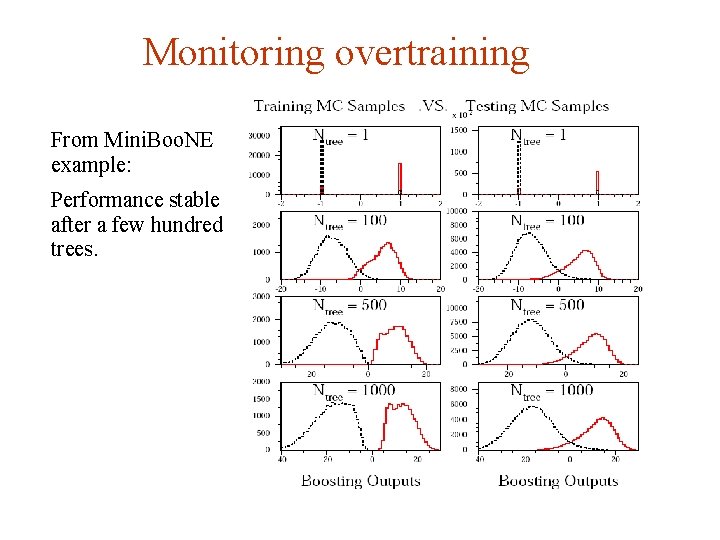
Monitoring overtraining From Mini. Boo. NE example: Performance stable after a few hundred trees. G. Cowan NEx. T Workshop, 2019 / GDC Lecture 2 page 46

Summary on multivariate methods Particle physics has used several multivariate methods for many years: linear (Fisher) discriminant neural networks naive Bayes and has in recent years started to use a few more: boosted decision trees support vector machines kernel density estimation k-nearest neighbour The emphasis is often on controlling systematic uncertainties between the modeled training data and Nature to avoid false discovery. Although many classifier outputs are "black boxes", a discovery at 5σ significance with a sophisticated (opaque) method will win the competition if backed up by, say, 4σ evidence from a cut-based method. G. Cowan NEx. T Workshop, 2019 / GDC Lecture 2 page 47