Sequential Logic Synthesis Giovanni De Micheli Integrated Systems

Sequential Logic Synthesis Giovanni De Micheli Integrated Systems Laboratory This presentation can be used for non-commercial purposes as long as this note and the copyright footers are not removed © Giovanni De Micheli – All rights reserved

Module 1 u Objective s Motivation and assumptions for sequential synthesis s Finite-state machine design and optimization (c) Giovanni De Micheli 2

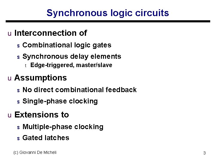
Synchronous logic circuits u Interconnection of s Combinational logic gates s Synchronous delay elements t Edge-triggered, master/slave u Assumptions s No direct combinational feedback s Single-phase clocking u Extensions to s Multiple-phase clocking s Gated latches (c) Giovanni De Micheli 3

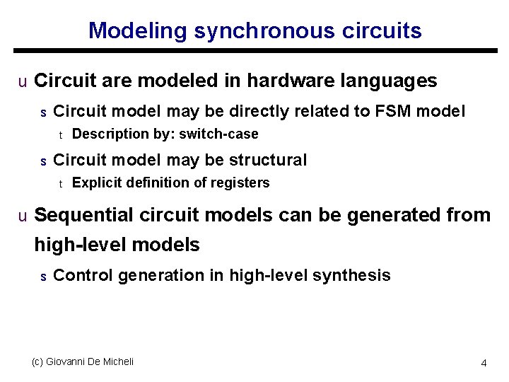
Modeling synchronous circuits u Circuit are modeled in hardware languages s Circuit model may be directly related to FSM model t s Description by: switch-case Circuit model may be structural t Explicit definition of registers u Sequential circuit models can be generated from high-level models s Control generation in high-level synthesis (c) Giovanni De Micheli 4

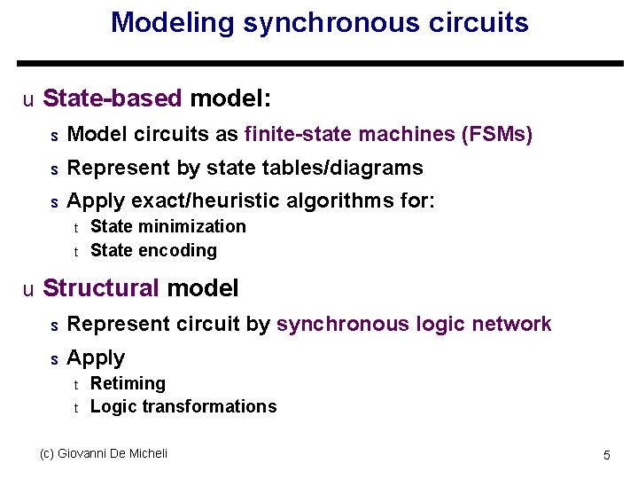
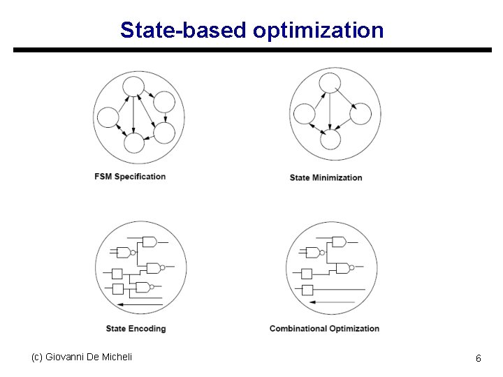
Modeling synchronous circuits u State-based model: s Model circuits as finite-state machines (FSMs) s Represent by state tables/diagrams s Apply exact/heuristic algorithms for: t t State minimization State encoding u Structural model s Represent circuit by synchronous logic network s Apply t t Retiming Logic transformations (c) Giovanni De Micheli 5

State-based optimization (c) Giovanni De Micheli 6

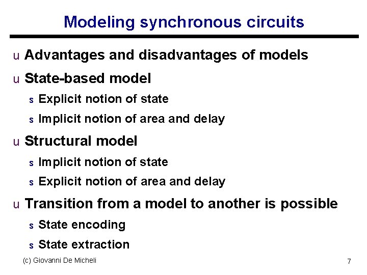
Modeling synchronous circuits u Advantages and disadvantages of models u State-based model s Explicit notion of state s Implicit notion of area and delay u Structural model s Implicit notion of state s Explicit notion of area and delay u Transition from a model to another is possible s State encoding s State extraction (c) Giovanni De Micheli 7

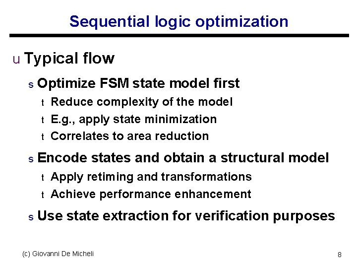
Sequential logic optimization u Typical flow s Optimize FSM state model first t s Encode states and obtain a structural model t t s Reduce complexity of the model E. g. , apply state minimization Correlates to area reduction Apply retiming and transformations Achieve performance enhancement Use state extraction for verification purposes (c) Giovanni De Micheli 8

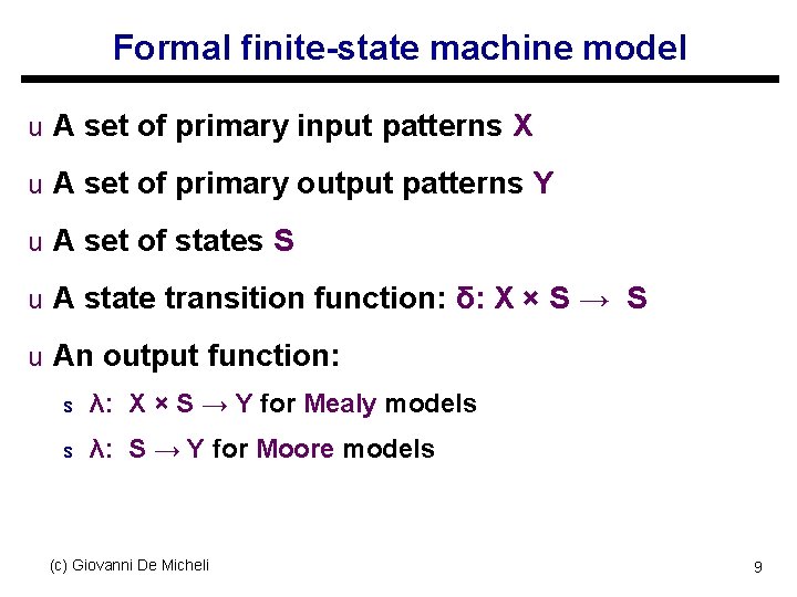
Formal finite-state machine model u A set of primary input patterns X u A set of primary output patterns Y u A set of states S u A state transition function: δ: X × S → S u An output function: s λ: X × S → Y for Mealy models s λ: S → Y for Moore models (c) Giovanni De Micheli 9

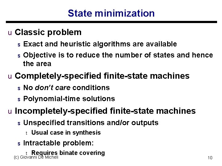
State minimization u Classic problem s Exact and heuristic algorithms are available s Objective is to reduce the number of states and hence the area u Completely-specified finite-state machines s s No don’t care conditions Polynomial-time solutions u Incompletely-specified finite-state machines s Unspecified transitions and/or outputs t s Usual case in synthesis Intractable problem: t Requires binate covering (c) Giovanni De Micheli 10

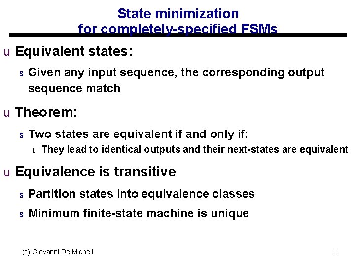
State minimization for completely-specified FSMs u Equivalent states: s Given any input sequence, the corresponding output sequence match u Theorem: s Two states are equivalent if and only if: t They lead to identical outputs and their next-states are equivalent u Equivalence is transitive s Partition states into equivalence classes s Minimum finite-state machine is unique (c) Giovanni De Micheli 11

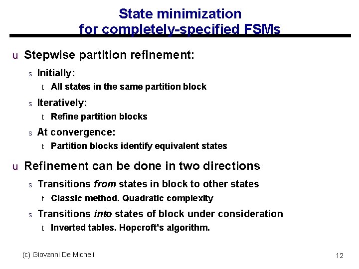
State minimization for completely-specified FSMs u Stepwise partition refinement: s Initially: t s Iteratively: t s All states in the same partition block Refine partition blocks At convergence: t Partition blocks identify equivalent states u Refinement can be done in two directions s Transitions from states in block to other states t s Classic method. Quadratic complexity Transitions into states of block under consideration t Inverted tables. Hopcroft’s algorithm. (c) Giovanni De Micheli 12

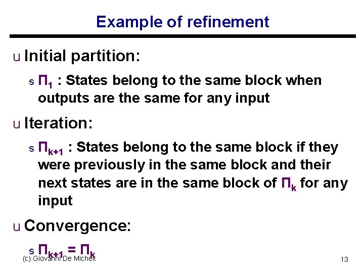
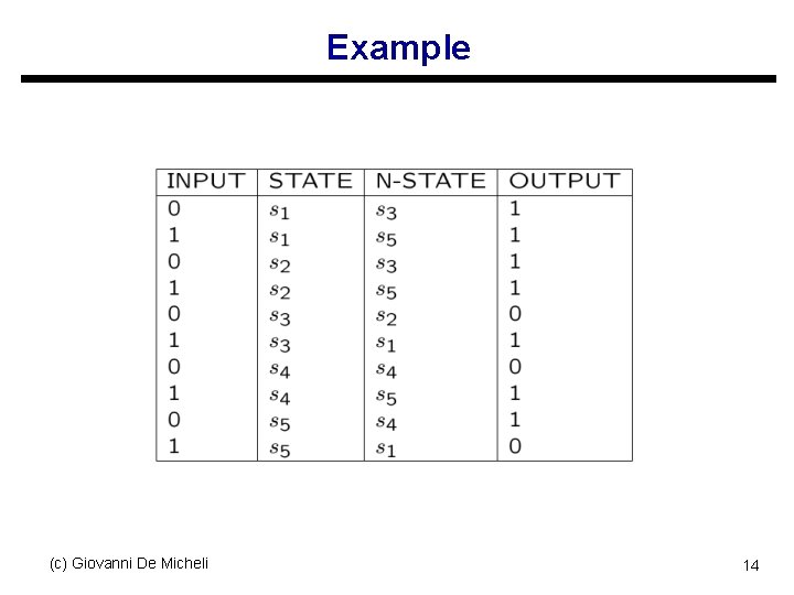
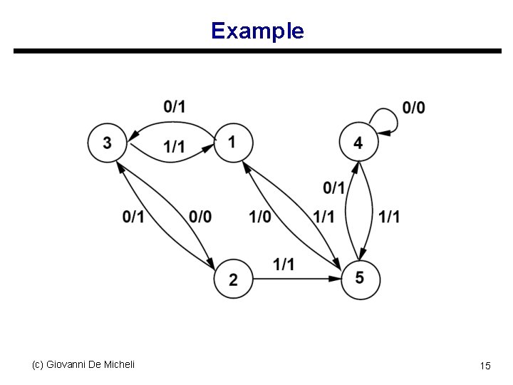
Example of refinement u Initial partition: s Π 1 : States belong to the same block when outputs are the same for any input u Iteration: s Πk+1 : States belong to the same block if they were previously in the same block and their next states are in the same block of Πk for any input u Convergence: Π = Π k+1 k (c) Giovanni De Micheli s 13

Example (c) Giovanni De Micheli 14

Example (c) Giovanni De Micheli 15

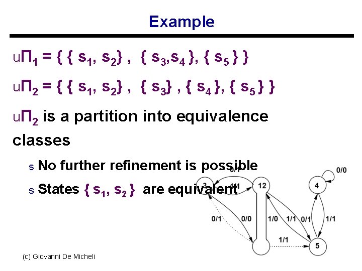
Example uΠ 1 = { { s 1, s 2} , { s 3, s 4 }, { s 5 } } uΠ 2 = { { s 1, s 2} , { s 3} , { s 4 }, { s 5 } } uΠ 2 is a partition into equivalence classes s No further refinement is possible s States { s 1, s 2 } are equivalent (c) Giovanni De Micheli 16

State minimization for incompletely-specified finite-state machines u Applicable input sequences s All transitions are specified u Compatible states s Given any applicable input sequence, the corresponding output sequence match u Theorem: s Two states are compatible if and only if: t They lead to identical outputs u t (when both are specified) And their next state is compatible u (when both are specified) (c) Giovanni De Micheli 17

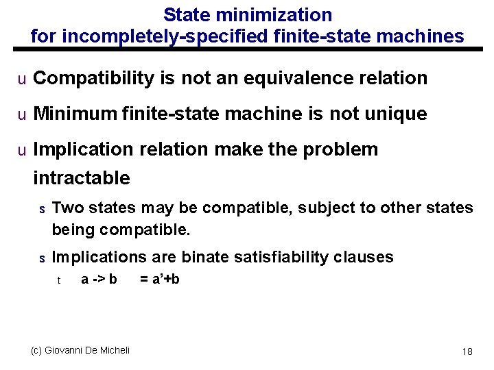
State minimization for incompletely-specified finite-state machines u Compatibility is not an equivalence relation u Minimum finite-state machine is not unique u Implication relation make the problem intractable s Two states may be compatible, subject to other states being compatible. s Implications are binate satisfiability clauses t a -> b (c) Giovanni De Micheli = a’+b 18

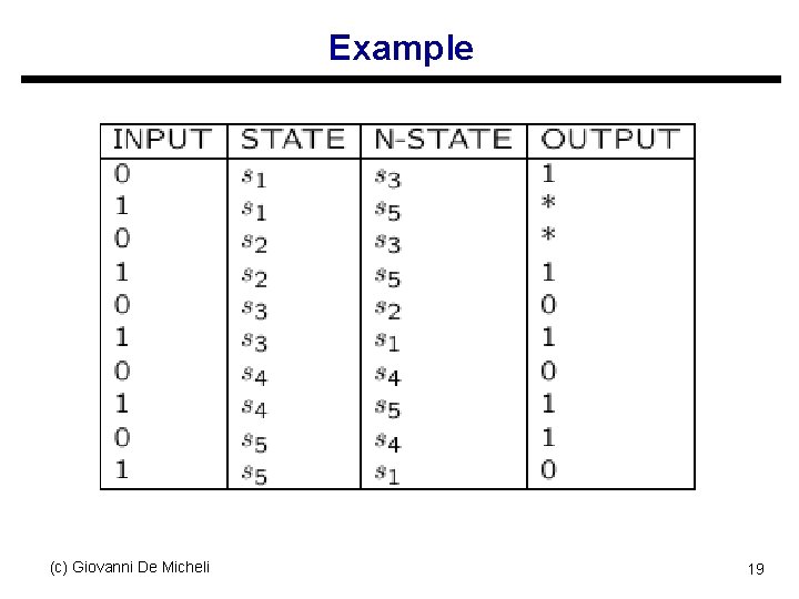
Example (c) Giovanni De Micheli 19

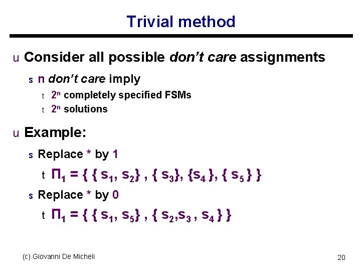
Trivial method u Consider all possible don’t care assignments s n don’t care imply t t 2 n completely specified FSMs 2 n solutions u Example: s Replace * by 1 t s Π 1 = { { s 1, s 2} , { s 3}, {s 4 }, { s 5 } } Replace * by 0 t Π 1 = { { s 1, s 5} , { s 2, s 3 , s 4 } } (c) Giovanni De Micheli 20

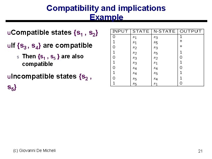
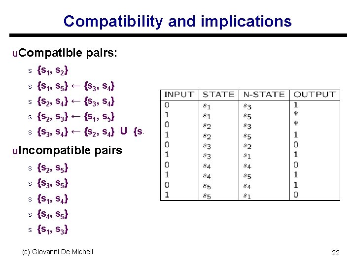
Compatibility and implications Example u. Compatible states {s 1 , s 2} u. If {s 3 , s 4} are compatible s Then {s 1 , s 5 } are also compatible u. Incompatible states {s 2 , s 5} (c) Giovanni De Micheli 21

Compatibility and implications u. Compatible pairs: s {s 1, s 2} s {s 1, s 5} ← {s 3, s 4} s {s 2, s 4} ← {s 3, s 4} s {s 2, s 3} ← {s 1, s 5} s {s 3, s 4} ← {s 2, s 4} U {s 1, s 5} u. Incompatible pairs s {s 2, s 5} s {s 3, s 5} s {s 1, s 4} s {s 4, s 5} s {s 1, s 3} (c) Giovanni De Micheli 22

Compatibility and implications u A class of compatible states is such that all state pairs are compatible u A class is maximal s If not subset of another class u Closure property s A set of classes such that all compatibility implications are satisfied u The set of maximal compatibility classes s Has the closure property s May not provide a minimum solution (c) Giovanni De Micheli 23

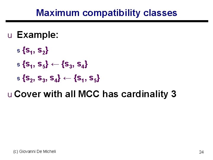
Maximum compatibility classes u Example: s {s 1, s 2} s {s 1, s 5} ← {s 3, s 4} s {s 2, s 3, s 4} ← {s 1, s 5} u Cover with all MCC has cardinality 3 (c) Giovanni De Micheli 24

Exact problem formulation u Prime compatibility classes: s Compatibility classes having the property that they are not subset of other classes implying the same (or subset) of classes u Compute all prime compatibility classes u Select a minimum number of prime classes s Such that all states are covered s All implications are satisfied u Exact solution requires binate cover u Good approximation methods exists s Stamina (c) Giovanni De Micheli 25

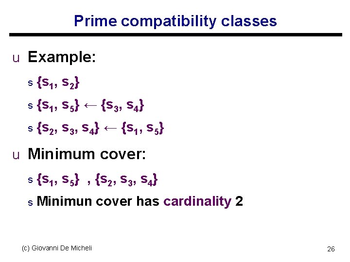
Prime compatibility classes u Example: s {s 1, s 2} s {s 1, s 5} ← {s 3, s 4} s {s 2, s 3, s 4} ← {s 1, s 5} u Minimum cover: s {s 1, s 5} , {s 2, s 3, s 4} s Minimun cover has cardinality 2 (c) Giovanni De Micheli 26

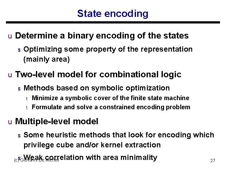
State encoding u Determine a binary encoding of the states s Optimizing some property of the representation (mainly area) u Two-level model for combinational logic s Methods based on symbolic optimization t t Minimize a symbolic cover of the finite state machine Formulate and solve a constrained encoding problem u Multiple-level model s Some heuristic methods that look for encoding which privilege cube and/or kernel extraction Weak correlation with area minimality (c)s. Giovanni De Micheli 27

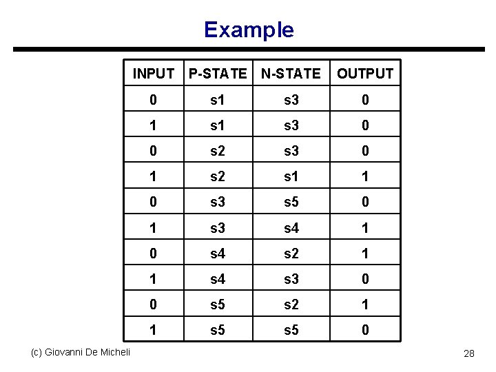
Example (c) Giovanni De Micheli INPUT P-STATE N-STATE OUTPUT 0 s 1 s 3 0 0 s 2 s 3 0 1 s 2 s 1 1 0 s 3 s 5 0 1 s 3 s 4 1 0 s 4 s 2 1 1 s 4 s 3 0 0 s 5 s 2 1 1 s 5 0 28

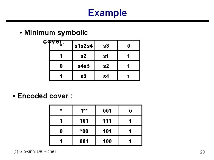
Example • Minimum symbolic cover: * s 1 s 2 s 4 s 3 0 1 s 2 s 1 1 0 s 4 s 5 s 2 1 1 s 3 s 4 1 * 1** 001 0 1 101 111 1 0 *00 101 1 1 001 100 1 • Encoded cover : (c) Giovanni De Micheli 29

Summary finite-state machine optimization u FSM optimization has been widely researched s Classic and newer approaches u State minimization and encoding correlate to area reduction s Useful, but with limited impact u Performance-oriented FSM optimization has mixed results s Performance optimization is usually done by structural methods (c) Giovanni De Micheli 30

Module 2 u Objective s Structural representation of sequential circuits s Retiming s Extensions (c) Giovanni De Micheli 31

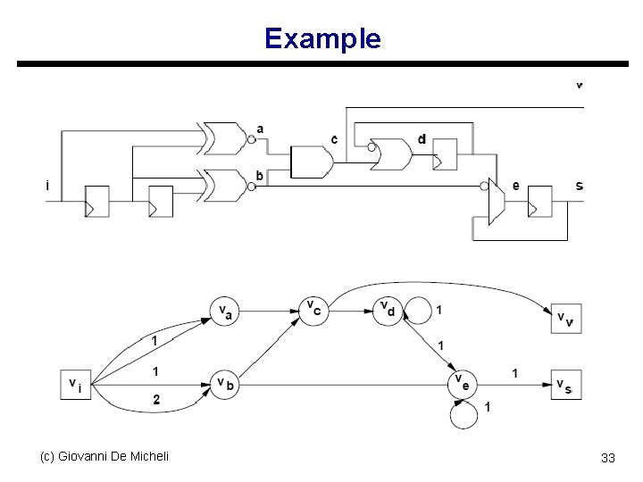
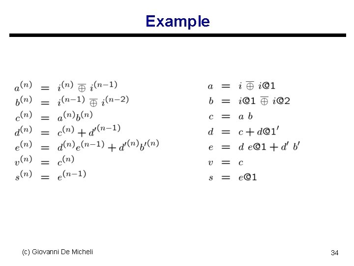
Structural model for sequential circuits u Synchronous logic network s Variables s Boolean equations s Synchronous delay annotation u Synchronous network graph s Vertices ↔ equations ↔ I/O, gates s Edges ↔ dependencies ↔ nets s Weights ↔ synchronous delays ↔ registers (c) Giovanni De Micheli 32

Example (c) Giovanni De Micheli 33

Example (c) Giovanni De Micheli 34

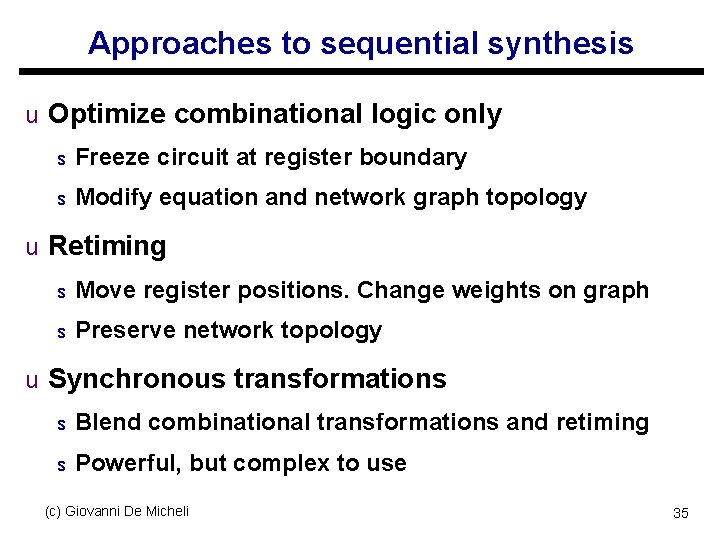
Approaches to sequential synthesis u Optimize combinational logic only s Freeze circuit at register boundary s Modify equation and network graph topology u Retiming s Move register positions. Change weights on graph s Preserve network topology u Synchronous transformations s Blend combinational transformations and retiming s Powerful, but complex to use (c) Giovanni De Micheli 35

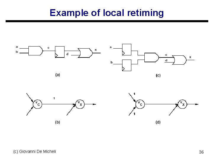
Example of local retiming (c) Giovanni De Micheli 36

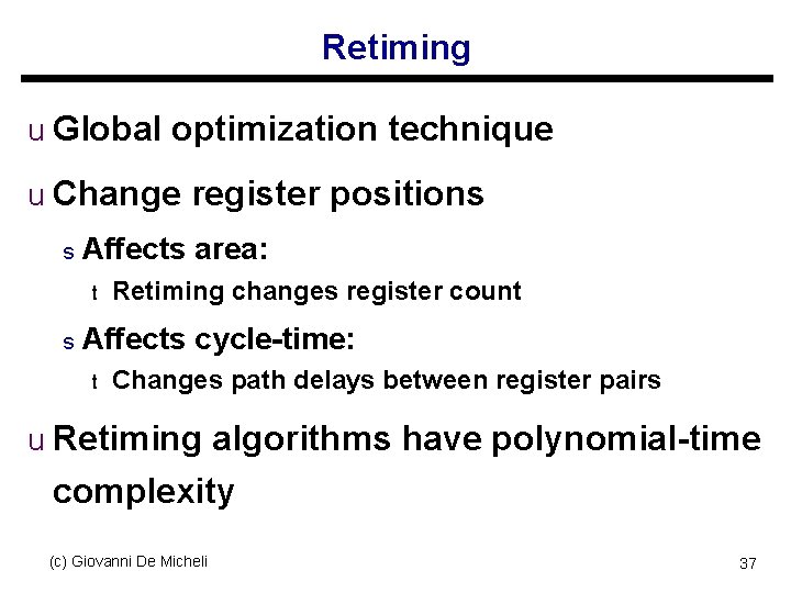
Retiming u Global optimization technique u Change register positions s Affects area: t s Retiming changes register count Affects cycle-time: t Changes path delays between register pairs u Retiming algorithms have polynomial-time complexity (c) Giovanni De Micheli 37

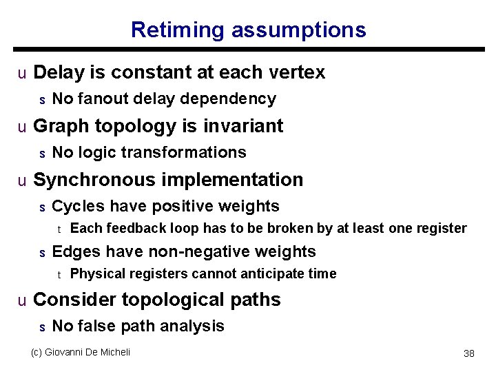
Retiming assumptions u Delay is constant at each vertex s No fanout delay dependency u Graph topology is invariant s No logic transformations u Synchronous implementation s Cycles have positive weights t s Each feedback loop has to be broken by at least one register Edges have non-negative weights t Physical registers cannot anticipate time u Consider topological paths s No false path analysis (c) Giovanni De Micheli 38

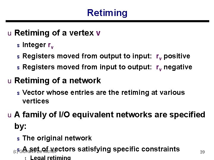
Retiming u Retiming of a vertex v s Integer rv s Registers moved from output to input: rv positive s Registers moved from input to output: rv negative u Retiming of a network s Vector whose entries are the retiming at various vertices u A family of I/O equivalent networks are specified by: s The original network A set of vectors satisfying specific constraints (c)s. Giovanni De Micheli t Legal retiming 39

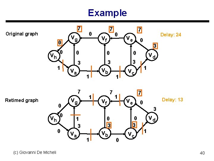
Example 7 Original graph 0 vh 0 1 vg 0 vh 0 0 (c) Giovanni De Micheli vf 0 7 ve 0 0 3 3 3 va 1 vg 1 vb 1 7 vf 1 Delay: 24 0 0 7 Retimed graph 0 7 3 vd 1 vc 7 ve Delay: 13 0 3 va 0 3 1 3 1 vb 0 vc vd 1 40

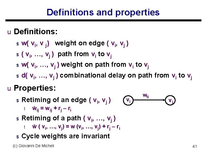
Definitions and properties u Definitions: s w( vi, v j) weight on edge ( vi, vj ) s ( vi, …, vj ) path from vi to vj s w( vi, …, vj ) weight on path from vi to vj s d( vi, …, vj ) combinational delay on path from vi to vj u Properties: s Retiming of an edge ( vi, vj ) t s vj ŵij = wij + rj – ri Retiming of a path ( vi, …, vj ) t s vi wij ŵ ( vi, …, vj) = w (vi, …, vj) + rj – ri Cycle weights are invariant (c) Giovanni De Micheli 41

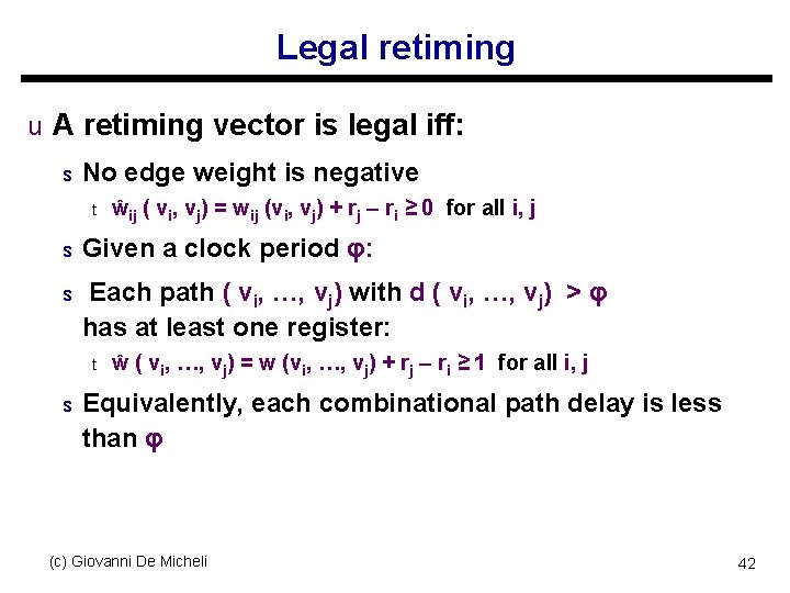
Legal retiming u A retiming vector is legal iff: s No edge weight is negative t ŵij ( vi, vj) = wij (vi, vj) + rj – ri ≥ 0 for all i, j s Given a clock period φ: s Each path ( vi, …, vj) with d ( vi, …, vj) > φ has at least one register: t s ŵ ( vi, …, vj) = w (vi, …, vj) + rj – ri ≥ 1 for all i, j Equivalently, each combinational path delay is less than φ (c) Giovanni De Micheli 42

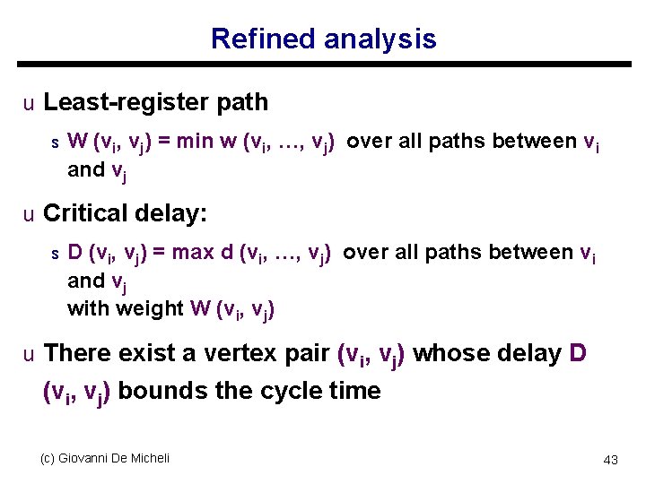
Refined analysis u Least-register path s W (vi, vj) = min w (vi, …, vj) over all paths between vi and vj u Critical delay: s D (vi, vj) = max d (vi, …, vj) over all paths between vi and vj with weight W (vi, vj) u There exist a vertex pair (vi, vj) whose delay D (vi, vj) bounds the cycle time (c) Giovanni De Micheli 43

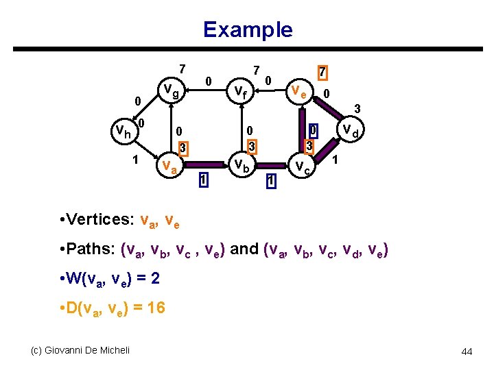
Example 7 0 vh vg vf 0 7 ve 0 3 0 1 0 7 va 0 3 0 3 1 vb 1 vc vd 1 • Vertices: va, ve • Paths: (va, vb, vc , ve) and (va, vb, vc, vd, ve) • W(va, ve) = 2 • D(va, ve) = 16 (c) Giovanni De Micheli 44

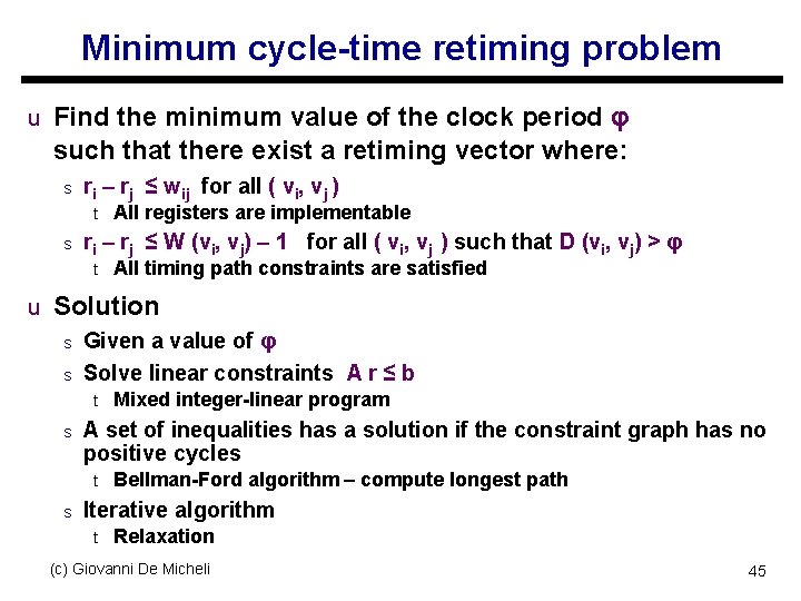
Minimum cycle-time retiming problem u Find the minimum value of the clock period φ such that there exist a retiming vector where: s ri – rj ≤ wij for all ( vi, vj ) t s All registers are implementable ri – rj ≤ W (vi, vj) – 1 for all ( vi, vj ) such that D (vi, vj) > φ t All timing path constraints are satisfied u Solution s Given a value of φ s Solve linear constraints A r ≤ b t s A set of inequalities has a solution if the constraint graph has no positive cycles t s Mixed integer-linear program Bellman-Ford algorithm – compute longest path Iterative algorithm t Relaxation (c) Giovanni De Micheli 45

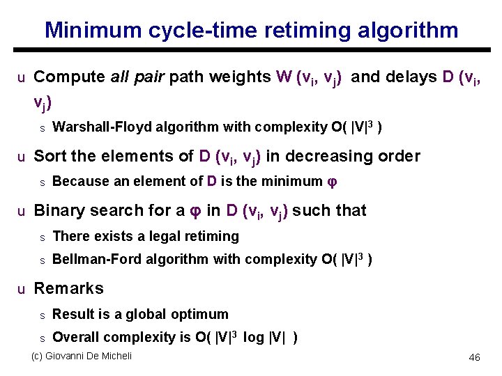
Minimum cycle-time retiming algorithm u Compute all pair path weights W (vi, vj) and delays D (vi, vj ) s Warshall-Floyd algorithm with complexity O( |V|3 ) u Sort the elements of D (vi, vj) in decreasing order s Because an element of D is the minimum φ u Binary search for a φ in D (vi, vj) such that s There exists a legal retiming s Bellman-Ford algorithm with complexity O( |V|3 ) u Remarks s Result is a global optimum s Overall complexity is O( |V|3 log |V| ) (c) Giovanni De Micheli 46

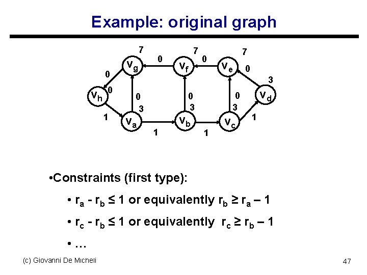
Example: original graph 7 0 vh 0 1 vg 0 7 vf 0 7 ve 0 3 va 0 3 0 3 1 vb 1 vc vd 1 • Constraints (first type): • ra - rb ≤ 1 or equivalently rb ≥ ra – 1 • rc - rb ≤ 1 or equivalently rc ≥ rb – 1 • … (c) Giovanni De Micheli 47

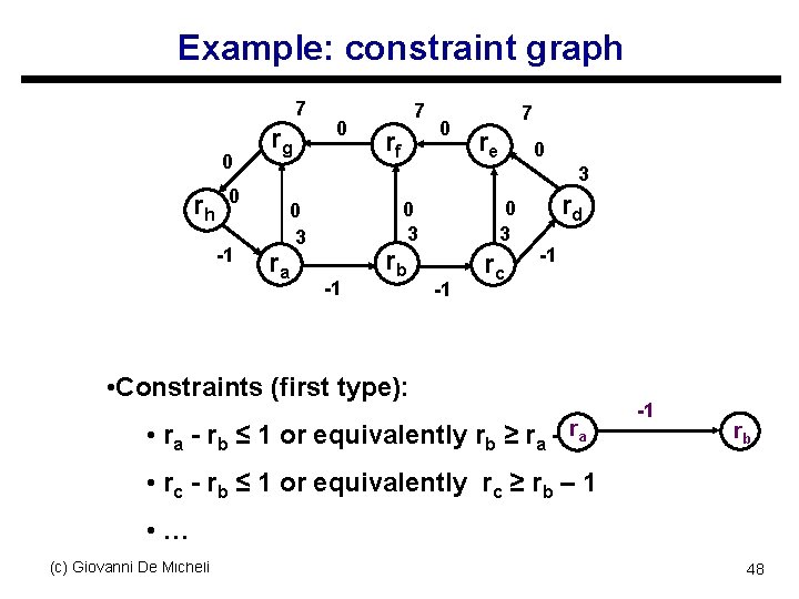
Example: constraint graph 7 0 rh rg rf 0 7 re 0 3 0 -1 0 7 ra 0 3 0 3 -1 rb -1 rc rd -1 • Constraints (first type): • ra - rb ≤ 1 or equivalently rb ≥ ra – r 1 a -1 rb • rc - rb ≤ 1 or equivalently rc ≥ rb – 1 • … (c) Giovanni De Micheli 48

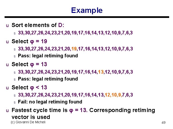
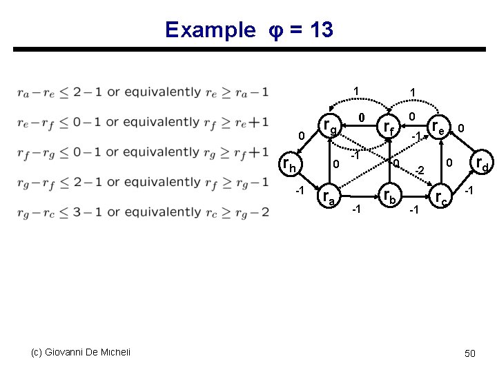
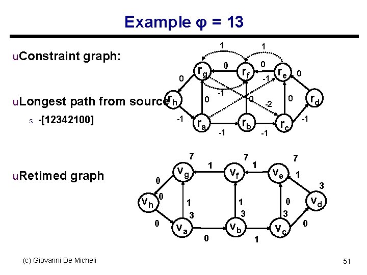
Example u Sort elements of D: s 33, 30, 27, 26, 24, 23, 21, 20, 19, 17, 16, 14, 13, 12, 10, 9, 7, 6, 3 u Select φ = 19 s 33, 30, 27, 26, 24, 23, 21, 20, 19, 17, 16, 14, 13, 12, 10, 9, 7, 6, 3 s Pass: legal retiming found u Select φ = 13 s 33, 30, 27, 26, 24, 23, 21, 20, 19, 17, 16, 14, 13, 12, 10, 9, 7, 6, 3 s Pass: legal retiming found u Select φ < 13 s 33, 30, 27, 26, 24, 23, 21, 20, 19, 17, 16, 14, 13, 12, 10, 9, 7, 6, 3 s Fail: no legal retiming found u Fastest cycle time is φ = 13. Corresponding retiming vector is used (c) Giovanni De Micheli 49

Example φ = 13 1 0 rh -1 (c) Giovanni De Micheli rg 0 ra 0 -1 -1 1 0 rf -1 0 rb -2 -1 re 0 rd 0 rc -1 50

Example φ = 13 1 u. Constraint graph: u. Longest path from sourcerh s 0 -1 -[12342100] ra 7 u. Retimed graph 0 vh 0 0 (c) Giovanni De Micheli 0 rg 0 vg 1 rf -1 vf -1 1 0 rd 0 -2 rb 7 re -1 0 -1 rc 7 ve 1 3 va 0 3 1 3 0 vb 1 vc vd 0 51

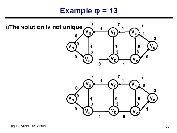
Example φ = 13 u. The solution is not unique 0 vh 0 0 7 vg vh 0 0 (c) Giovanni De Micheli vf 1 7 ve 1 3 va 0 vg 1 vb 1 7 vf vd 0 3 1 3 7 0 1 7 1 0 vc 7 ve 0 3 va 0 3 1 3 1 vb 0 vc vd 1 52

Relaxation-based retiming u Most common algorithm for retiming s Avoids storage of matrices W and D s Applicable to large circuits u Rationale s Search for decreasing φ in fixed step t s Use efficient method to determine legality t s Look for values of φ compatible with peripheral circuits Network graph is often very sparse Can be coupled with topological timing analysis (c) Giovanni De Micheli 53

Relaxation-based retiming u Start with a given cycle-time φ u Look for paths with excessive delays u Make such paths shorter s By bringing the terminal register closer s Some other paths may become longer s Namely, those path whose tail has been moved u Use an iterative approach (c) Giovanni De Micheli 54

Relaxation-based retiming u Define data ready time at each node s Total delay from register boundary u Iterative approach s Find vertices with data ready > φ s Retime these vertices by 1 u Algorithm properties s If at some iteration there is no vertex with data ready > φ, a legal retiming has been found s If a legal retiming is not found in |V| iterations, then no legal retiming exists for that φ (c) Giovanni De Micheli 55

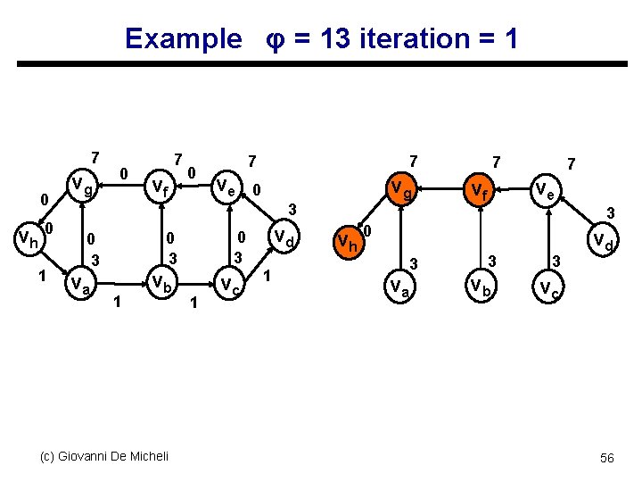
Example φ = 13 iteration = 1 7 0 vh 0 1 vg 0 7 vf 0 7 ve 7 vg 0 3 va 0 3 0 3 1 vb (c) Giovanni De Micheli 1 vc vd 1 7 7 ve vf 3 vh 0 va 3 3 vb 3 vd vc 56

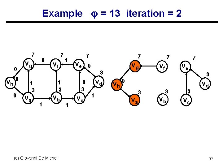
Example φ = 13 iteration = 2 7 0 vh 0 0 vg 0 7 vf 1 7 ve 7 vg 0 3 va 0 3 1 3 1 vb (c) Giovanni De Micheli 1 vc vd 1 7 7 ve vf 3 vh 0 va 3 3 vb 3 vd vc 57

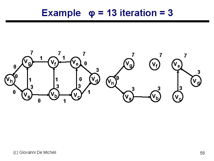
Example φ = 13 iteration = 3 7 0 vh 0 0 vg 1 7 vf 1 7 ve 7 vg 0 3 va 0 3 1 3 0 vb (c) Giovanni De Micheli 1 vc vd 1 7 7 ve vf 3 vh 0 va 3 3 vb 3 vd vc 58

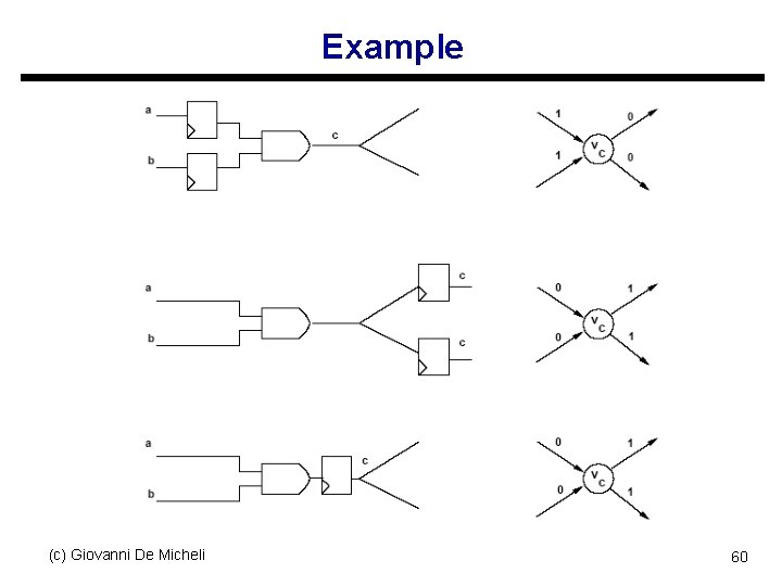
Retiming for minimum area u Find a retiming vector that minimizes the number of registers u Simple area modeling s Every edge with a positive weight denotes registers s Total register area is proportional to the sum of all weights u Register sharing model s Every set of positively-weighted edges with common tail is realized by a shift register with taps Total register area is proportional to the sum, over all vertices, of the maxima of weights on outgoing (c) Giovanni De Micheli 59 edges s

Example (c) Giovanni De Micheli 60

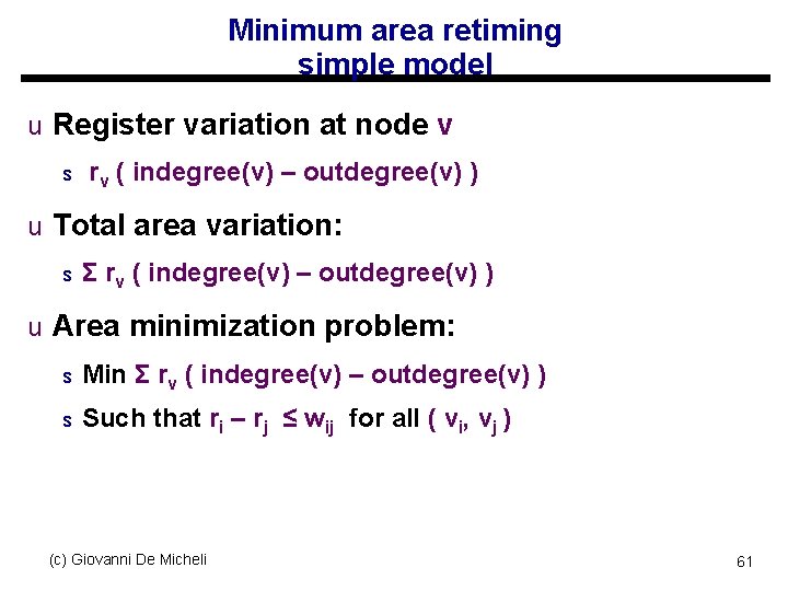
Minimum area retiming simple model u Register variation at node v s rv ( indegree(v) – outdegree(v) ) u Total area variation: s Σ rv ( indegree(v) – outdegree(v) ) u Area minimization problem: s Min Σ rv ( indegree(v) – outdegree(v) ) s Such that ri – rj ≤ wij for all ( vi, vj ) (c) Giovanni De Micheli 61

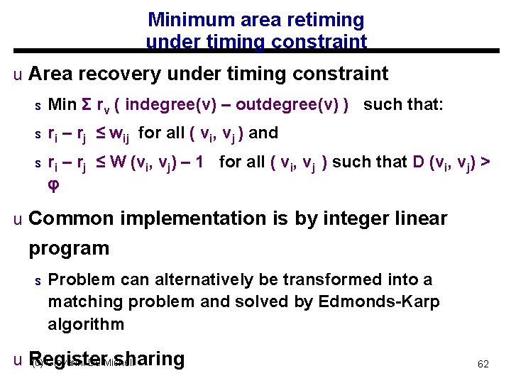
Minimum area retiming under timing constraint u Area recovery under timing constraint s Min Σ rv ( indegree(v) – outdegree(v) ) such that: s ri – rj ≤ wij for all ( vi, vj ) and s ri – rj ≤ W (vi, vj) – 1 for all ( vi, vj ) such that D (vi, vj) > φ u Common implementation is by integer linear program s Problem can alternatively be transformed into a matching problem and solved by Edmonds-Karp algorithm u Register sharing (c) Giovanni De Micheli 62

Other problems related to retiming u Retiming pipelined circuits s Balance pipe stages by using retiming s Trade-off latency versus cycle time u Peripheral retiming s Use retiming to move registers to periphery of a circuit s Restore registers after optimizing combinational logic u Wire pipelining s Use retiming to pipeline interconnection wires s Model sequential and combinational macros Consider wire delay and buffering (c)s. Giovanni De Micheli 63

Summary of retiming u Sequential optimization technique for: s Cycle time or register area u Applicable to s Synchronous logic networks s Architectural models of data paths t s Vertices represent complex (arithmetic) operators Exact algorithm in polynomial time u Extension and issues s Delay modeling s Network granularity (c) Giovanni De Micheli 64

Module 3 u Objective s Relating state-based and structural models s State extraction (c) Giovanni De Micheli 65

Relating the sequential models u State encoding s Maps a state-based representation into a structural one u State extraction s Recovers the state information from a structural model u Remark s A circuit with n registers may have 2 n states s Unreachable states (c) Giovanni De Micheli 66

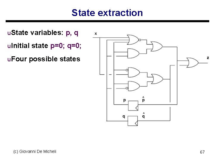
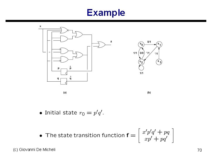
State extraction u. State variables: p, q u. Initial state p=0; q=0; u. Four possible states (c) Giovanni De Micheli 67

State extraction u Reachability analysis s Given a state, determine which states are reachable for some inputs s Given a state subset, determine the reachable state subset s Start from an initial state s Stop when convergence is reached u Notation: s A state (or a state subset) is represented by an expression over the state variables Implicit representation (c)s. Giovanni De Micheli 68

Reachability analysis u State transition function: f u Initial state: r 0 u States reachable from r 0 s Image of r 0 under f u States reachable from set rk s Image of rk under f u Iteration s rk+1 = rk U ( image of rk under f) u Convergence s rk+1 = rk for some k (c) Giovanni De Micheli 69

Example (c) Giovanni De Micheli 70

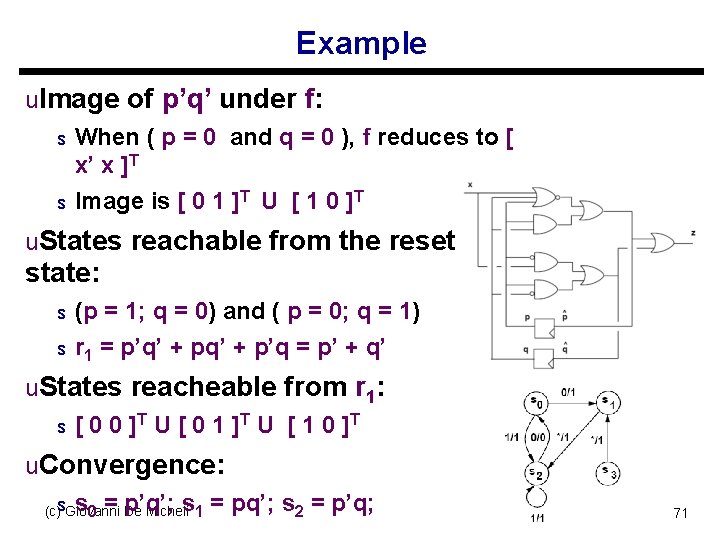
Example u. Image of p’q’ under f: s s When ( p = 0 and q = 0 ), f reduces to [ x’ x ]T Image is [ 0 1 ]T U [ 1 0 ]T u. States reachable from the reset state: s s (p = 1; q = 0) and ( p = 0; q = 1) r 1 = p’q’ + p’q = p’ + q’ u. States reacheable from r 1: s [ 0 0 ]T U [ 0 1 ] T U [ 1 0 ] T u. Convergence: s = p’q’; s = pq’; s 2 = p’q; (c)s. Giovanni De Micheli 1 0 71

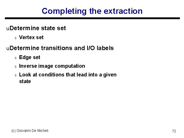
Completing the extraction u. Determine state set s Vertex set u. Determine transitions and I/O labels s Edge set s Inverse image computation s Look at conditions that lead into a given state (c) Giovanni De Micheli 72

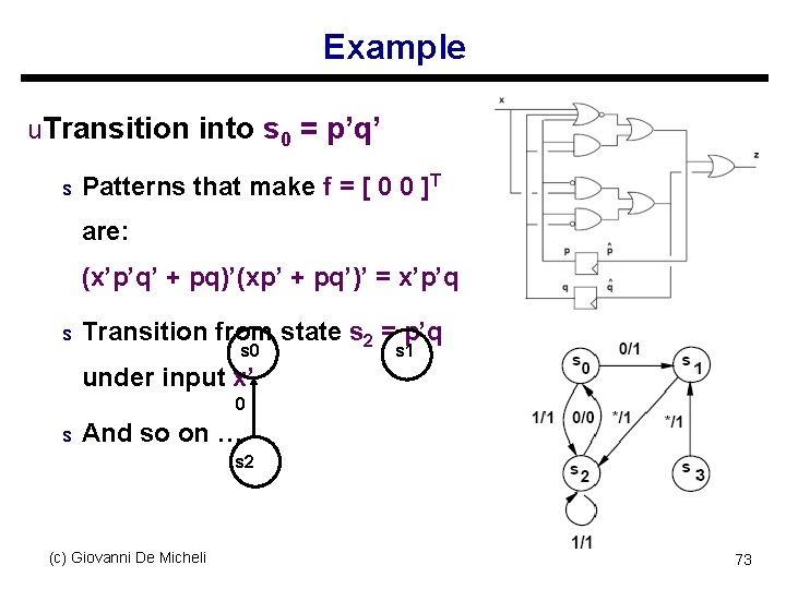
Example u. Transition into s 0 = p’q’ s Patterns that make f = [ 0 0 ]T are: (x’p’q’ + pq)’(xp’ + pq’)’ = x’p’q s Transition from state s 2 = p’q s 0 s 1 under input x’ 0 s And so on … s 2 (c) Giovanni De Micheli 73

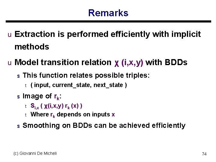
Remarks u Extraction is performed efficiently with implicit methods u Model transition relation χ (i, x, y) with BDDs s This function relates possible triples: t s Image of rk: t t s ( input, current_state, next_state ) Si, x ( χ(i, x, y) rk (x) ) Where rk depends on inputs x Smoothing on BDDs can be achieved efficiently (c) Giovanni De Micheli 74

Summary u State extraction can be performed efficiently to: s Apply state-based optimization techniques s Apply verification techniques u State extraction is based on forward and backward state space traversal: s Represent state space implicitly with BDDs s Important to manage the space size, which grows exponentially with the number of registers (c) Giovanni De Micheli 75