Semantically Equivalent Formulas Let and be formulas of

Semantically Equivalent Formulas • Let Φ and ψ be formulas of propositional logic. We say that Φ and ψ are semantically equivalent iff Φ╞ψ ψ╞Φ hold. In that case we write Φ ≡ ψ. Further, we call Φ valid if ╞Φ holds. 1

Examples of equivalent formulas • • p → q ≡ ¬p q p → q ≡ ¬q → ¬p p q → p ≡ r ¬r p q → r ≡ p → (q →r) 2

Lemma • Given propositional logic formulas Φ 1, Φ 2, …, Φn, ψ, we have Φ 1, Φ 2, …, Φn ╞ ψ iff ╞ Φ 1 →(Φ 2 → (Φ 3 → … → (Φn → ψ))) 3

Literal • A literal is either an atom p or the negation of an atom ¬p. 4
 • A formula Φ is in conjunctive normal form (CNF)")
Conjunctive Normal Form (CNF) • A formula Φ is in conjunctive normal form (CNF) if it is of the form ψ1 ψ2 …. ψn for some n ≥ 1, such that ψi is a literal, or a disjunction of literal, for all 1 ≤ i ≤ n. 5
 (¬p r) q • (p r)")
Examples for CNF formulas • (¬q p r) (¬p r) q • (p r) (¬p r) (p ¬r) 6

Lemma • A disjunction of literals L 1 L 2 …. Lm is valid (i. e. , ╞ L 1 L 2 …. Lm) iff there are 1 ≤ i, j ≤ m such that Li is ¬Lj. 7

Satisfiable formulas • Given a formula Φ in a propositional logic, we say that Φ is satisfiable if there exists an assignment of truth values to its propositional atoms such that Φ is true. 8

Proposition • Let Φ be a formula of propositional logic. Then Φ is satisfiable iff ¬Φ is not valid. 9
 /* pre-condition: Φ implication free and in NNF*/ /* post-condition: CNF(Φ) computes")
function CNF(Φ) /* pre-condition: Φ implication free and in NNF*/ /* post-condition: CNF(Φ) computes an equivalent CNF for Φ */ begin function case Φ is a literal : return Φ Φ is Φ 1 Φ 2: return CNF(Φ 1) CNF(Φ 2) Φ is Φ 1 Φ 2: return DISTR(CNF(Φ 1), CNF(Φ 2) ) end case end function 10
: /* pre-condition: η 1 and η 2 are in")
function DISTR(η 1, η 2): /* pre-condition: η 1 and η 2 are in CNF */ /* post-condition: DISTR(η 1, η 2) computes a CNF for η 1 η 2 */ begin function case η 1 is η 11 η 12 : return DISTR(η 11 , η 2) DISTR(η 12 , η 2) η 2 is η 21 η 22 : return DISTR(η 1 , η 21) DISTR(η 1 , η 22) otherwise (= no conjunction): return η 1 η 2 end case end function 11
 /* pre-condition: Φ is implication free */ /* post-condition: NNF(Φ) computes a")
function NNF(Φ) /* pre-condition: Φ is implication free */ /* post-condition: NNF(Φ) computes a NNF for Φ */ begin function case Φ is a literal : return Φ Φ is ¬¬Φ 1 : return NNF(Φ 1) Φ is Φ 1 Φ 2 : return NNF(Φ 1) NNF(Φ 2) Φ is ¬(Φ 1 Φ 2) : return NNF(¬Φ 1 ¬Φ 2) end case end function 12
 IMPL_FREE Φ = ¬ IMPL_FREE")
Φ = ¬p q → p (r → q) IMPL_FREE Φ = ¬ IMPL_FREE (¬p q ) IMPL_FREE (p (r → q)) = ¬((IMPL_FREE ¬p ) (IMPL_FREE q )) IMPL_FREE (p (r → q)) = ¬((¬p ) IMPL_FREE q ) IMPL_FREE (p (r → q)) = ¬ (¬p q ) ((IMPL_FREE (p) IMPL_FREE (r → q)) = ¬ (¬p q ) (p (¬ (IMPL_FREE r) IMPL_FREE (q))) = ¬ (¬p q ) (p (¬ r q)) 13
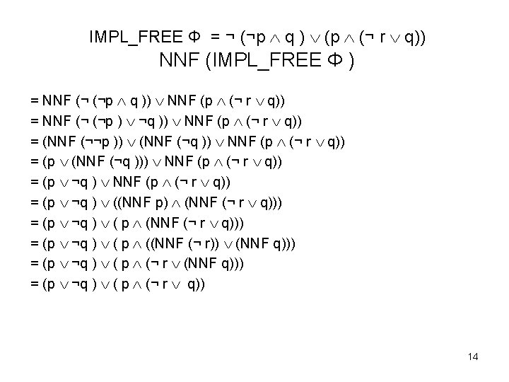
 = (p ¬q ) ( p (¬ r q)) CNF(NNF (IMPL_FREE")
NNF (IMPL_FREE Φ) = (p ¬q ) ( p (¬ r q)) CNF(NNF (IMPL_FREE Φ)) = CNF ((p ¬q ) ( p (¬r q))) = DISTR ( CNF (p ¬q ), CNF (p (¬ r q))) = DISTR (p ¬q , p (¬ r q)) = DISTR (p ¬q , p) DISTR (p ¬q , ¬ r q) = (p ¬q p) (p ¬q ¬ r q) 15

Horn Formula Φ • is a formula Φ of propositional logic if it is of the form ψ1 ψ2. . . ψn for some n ≥ 1 such that ψi is of the form p 1 p 2. . . pki → qi for some ki ≥ 1, where p 1, …, pki, qi are atoms, ┴ or T. We call such ψi a Horn clause. 16
 (q r → p)")
Examples of Horn formulas • (p q s → p) (q r → p) (p s → s) • (p q s → ┴) (q r → p) (T → s) • (p 2 p 3 p 5 → p 13) (T→ p 2) (p 5 p 11 → ┴) 17
 (q r →")
Examples of non-Horn formulas • • (p q s → ¬p) (q r → p) (p s → s) (p q s → ┴) (¬q r → p) (T → s) (p 2 p 3 p 5 → p 13 p 27) (T→ p 2) (p 5 p 11 → ┴) (p 2 p 3 p 5 → p 13 ) (T→ p 2) (p 5 p 11 ┴) 18
 /* Pre-condition : Φ is a Horn formula*/ /* Post-condition : HORN(Φ)")
function HORN(Φ) /* Pre-condition : Φ is a Horn formula*/ /* Post-condition : HORN(Φ) decides the satisfiability for Φ */ begin function mark all atoms p where T → p is a sub-formula of Φ; while there is a sub-formula p 1 p 2. . . pki → qi of Φ such that all pj are marked but qi is not do if qi ≡ ┴ then return ‘unsatisfiable’ else mark qi for all such subformulas end while return ‘satisfiable’ end function 19

Theorem • The algorithm HORN is correct for the satisfiability decision problem of Horn formulas and has no more than n cycles in its while-loop if n is the number of atoms in Φ. HORN always terminates on correct input. 20

Kripke structure Let AP be a set of atomic propositions. A Kripke structure M over AP is a four tuple M= (S, S 0, R, L) where 1. S is a finite set of states 2. S 0 S is the set of initial states. 3. R S × S is a transition relation that must be total, that is for every state s S there is a state s’ S such that R (s, s’). 4. L: S 2 AP is a function that labels each state with the set of atomic proposition in that state. A path in the structure M from a state s is an infinite sequence of states ω = s 0 s 1 s 2 … such that s 0 = s and R (si, si+1) holds for all i ≥ 0. 21

First order representation of Kipke structures • We use interpreted first order formulas to describe concurrent systems. • We usual logical connectives (and , or , implies , not , and so on) and universal ( ) and existential ( ) quantifications. • Let V = {v 1, …, vn} be the set of system variables. We assume that the variables in V range over a finite set D. • A valuation for V is a function that associated a value in D with each variable v in V. Thus, s is a valuation for V when s: V D. • A state of a concurrent system can be viewed as a valuation for the set of its variables V. • Let V’ = {v’ 1, …, v’n}. We think of the variables in V as present state variables and the variables in V’ as next state variables. 22
")
First order representation of Kipke structures Let M = (S, S 0, R, L) be a Kripke structure. • S is the set of all valuations for all variables of the system which can be described by a proposition S. Usually, S = True. • The set of initial states S 0 can be described by a proposition (on the set of variables) S 0. • R can be described by a proposition R such that for any two states s and s’, R(s, s’) holds if R evaluates to True when each variable v is assigned the value s(v) and each variable v’ is assigned the value s(v’). • The labeling function L: S 2 AP is defined so that L(s) is the subset of all atomic propositions true in s which can be described by some appropriate proposition. 23

A simple example We consider a simple system with variables x and y that range over D = {0, 1}. Thus, a valuation for the variables x and y is just a pair (d 1, d 2) D × D where d 1 is the value for x and d 2 is the value for y. The system consists of one transition x : = (x +y) mod 2, Which starts from the state in which x = 1 and y = 1. 24
 mod 2 • S")
A simple example with transition x : = (x +y) mod 2 • S = True • S 0 (x, y) ≡ x = 1 y = 1 • R (x, y, x’, y’) ≡ x’ = (x +y) mod 2 y’ = y 25
 mod 2 The Kripke")
A simple example with transition x : = (x +y) mod 2 The Kripke structure M = (S, S 0, R, L) for this system is simply: • S = D × D. • S 0 = {(1, 1)} • R = {((1, 1), (0, 1)), ((0, 1), (1, 1)), ((1, 0), (1, 0)), ((0, 0), (0, 0))}. • L(1, 1) = {x =1, y = 1}, L(0, 1) = {x =0, y = 1}, L(1, 0) = {x =1, y = 0}, L(0, 0) = {x =0, y = 0}. The only path in the Kripke structure that starts in the initial state is (1, 1) (0, 1) …. 26

Concurrent systems • A concurrent system consists of a set of components that execute together. • Normally, the components have some means of communicating with each other. 27

Modes of execution We will consider two modes of execution: Asynchronous or interleaved execution, in which only one component makes a step at a time, and synchronous execution, in which all of the components make a step at the same time 28

Modes of communication • We will also distinguish three modes of communication. Components can either communicate by changing the value of shared variables or by exchanging messages using queues or some handshaking protocols. 29

A modulo 8 counter 30

Synchronous circuit A modulo 8 counter The transitions of the circuit are given by • v’ 0 = v 0 • v’ 1 = v 0 v 1 • v’ 2 = (v 0 v 1) v 2 • R 0 (v, v’) ≡ (v’ 0 ↔ v 0) • R 1 (v, v’) ≡ (v’ 1 ↔ v 0 v 1) • R 2 (v, v’) ≡ (v’ 2 ↔ (v 0 v 1) v 2) • R (v, v’) ≡ R 0 (v, v’) R 1 (v, v’) R 2 (v, v’) 31

Synchronous circuit General case • • Let V = {v 0, …. , vn-1} and V’ = {v’ 0, …. , v’n-1} Let v’i = fi (V), 1= 0, …, n-1. Define Ri (v, v’) ≡ ( v’i ↔ fi (V)). Then, the transition relation can be described as R (v, v’) ≡ R 0 (v, v’) … Rn-1 (v, v’). 32

Asynchronous circuit General case • In this case, the transition relation can be described as R (v, v’) ≡ R 0 (v, v’) … Rn-1 (v, v’), Where Ri (v, v’) ≡ ( v’i ↔ fi (V)) j ≠ i (v’j ↔ vj )). 33

Example • Let V = {v 0, v 1}, v’ 0 = v 0 v 1 and v’ 1 = v 0 v 1. • Let s be a state with v 0 = 1 v 1 = 1. • For the synchronous model, the only successor of s is the state v 0 = 0 v 1 = 0. • For the asynchronous model, the state s has two successors: • 1. v 0 = 0 v 1 = 1 ( the assignment to v 0 is taken first). • 2. v 0 = 1 v 1 = 0 ( the assignment to v 1 is taken first). 34

Labeled program Given a statement P, the labeled statement PL is defined as follows: • If P is not a composite statement then P = PL. . • If P = P 1; P 2 then PL = P 1 L ; l’’ : P 2 L. • If P = if b then P 1 else P 2 end if, then PL = if b then l 1 : P 1 L else l 2 : P 2 L end if. • If P = while b do P 1 end while, then PL = while b do l 1 : P 1 L end while. 35

Some assumptions • We assume that P is a labeled statement and that the entry and exit points of P are labeled by m and m’, respectively. • Let pc be a special variable called the program counter that ranges over the set of program labels and an additional value ┴ called the undefined value. • Let V denote the set of program variables, V’ the set of primed variables for V, and pc’ the primed variables for pc. • Let same (Y) = y ε Y (y’ = y). 36
 on")
The set of initial states of P • Given some condition pre (V) on the initial variables for P, S 0 (V, pc) ≡ pre (V) pc = m. 37
 describes the set of")
The transition relation for P • C (l, P, l’) describes the set of transitions in P as a disjunction of all transitions in the set. • Assignment: C ( l, v ← e, l’) ≡ pc = l pc’ = l’ v’ = e same (V {v}) • Skip: C ( l, skip, l’) ≡ pc = l pc’ = l’ same (V) • Sequential composition: C ( l, P 1; l’’ : P 2, l’) ≡ C ( l, P 1, l’’) C ( l’’, P 2, l’) 38
 • Conditional: C (l, if b then l")
The transition relation for P (continued) • Conditional: C (l, if b then l 1: P 1 else l 2 : P 2 end if, l’) is the disjunction of the following formulas: • pc = l pc’ = l 1 b same (V) • pc = l pc’ = l 2 b same (V) • C (l 1, P 1, l’) • C (l 2, P 2, l’) 39
 • While: C (l, while b do l")
The transition relation for P (continued) • While: C (l, while b do l 1 : P 1 end while, l’) is the disjunction of the following formulas: • pc = l pc’ = l 1 b same (V) • pc = l pc’ = l’ b same (V) • C (l 1, P 1, l) 40

Concurrent programs • A concurrent program consists of a set of processes that can be executed in parallel. A process is a sequential program. • Let Vi be the set of variables that can be changed by process Pi. V is the set of all program variables. • pci is the program counter of process Pi. PC is the set of all program counters. • A concurrent program has the form cobegin P 1 || P 2 … || Pn coend where P 1, …, Pn are processes. 41

Labeling transformation • We assume that no two labels are identical and that the entry and exit points of P are labeled m and m’, respectively. • If P = cobegin P 1 || P 2 … || Pn coend, then PL = cobegin l 1 : P 1 L l’ 1 || l 2 : P 2 L l’ 2 || … || ln : Pn. L l’n coend. 42
 ≡ pre (V)")
The set of initial states of P S 0 (V, pc) ≡ pre (V) pc = m i = 1, … n (pci = ┴ ) 43

The transition relation for P C (l, cobegin l 1 : P 1 L l’ 1 || … || ln : Pn. L l’n coend, l’) Is the disjunction of three formulas: • pc = l pc’ 1 = l 1 … pc’n = ln pc’ = ┴ • pc = ┴ pc 1 = l’ 1 … pcn = l’n pc’ = l’ • i = 1, … n (pc’i = ┴) (C (li, Pi, l’i) (same (V Vi) same (PC {pci})) 44
, l’) is a disjunction")
Shared variables • Wait: • • C (l, wait (b), l’) is a disjunction of the following two formulas: (pci = l pc’i = l b same (Vi)) (pci = l pc’i = l’ b same (Vi)) • Lock (v) (= wait (v = 0)): • • C (l, lock (v), l’) is a disjunction of the following two formulas: (pci = l pc’i = l v = 1 same (Vi)) (pci = l pc’i = l’ v = 0 v’ = 1 same (Vi {v})) • Unlock (v): C (l, unlock (v), l’) ≡ pci = l pc’i = l’ v’ = 0 same (Vi {v}) 45

A simple mutual exclusion program P = m: cobegin P 0 || P 1 coend m’ P 0 : : l 0 : while True do NC 0 : wait (turn = 0); CR 0 : turn : =1; end while; l’ 0 P 1 : : l 1 : while True do NC 1 : wait (turn = 1); CR 1 : turn : = 0; end while; l’ 1 46

Kripke structure • pc takes values in the set { m, m’, ┴ }. • pci takes values in the set { li, l’i, NCi, CRi, ┴ }. • V = V 0 = V 1 = {turn}. • PC = {pc, pc 0, pc 1}. 47
 ≡ pc")
The set of initial states of P • S 0 (V, PC) ≡ pc = m pc 0 = ┴ pc 1 = ┴. 48
 is the disjunction")
The transition relation for P • R (V, PC, V’, PC’) is the disjunction of the following four formulas: • pc = m pc’ 0 = l 0 pc’ 1 = l 1 pc’ = ┴. • pc 0 = l’ 0 pc 1 = l’ 1 pc’ = m’ pc’ 0 = ┴ pc’ 1 = ┴. • C (l 0, P 0, l’ 0) same (pc, pc 1). • C (l 1, P 1, l’ 1) same (pc, pc 0). 49

The transition relation of Pi • • • For each process Pi, C (li, Pi, l’i) is the disjunction of: pci = li pc’i = NCi True same (turn) pci = NCi pc’i = CRi turn = i same (turn) pci = CRi pc’i = li turn’ = (i+1) mod 2 pci = NCi pc’i = NCi turn ≠ i same (turn) pci = li pc’i = l’i False same (turn) 50

turn = 0 ┴, ┴ turn = 1 ┴, ┴ turn = 0 l 0, l 1 turn = 0 l 0, NC 1 turn = 0 turn = 1 l 0, l 1 turn = 0 l 1, NC 0 turn = 0 CR 0, l 1 NC 0, NC 1 turn = 0 CR 0, NC 1 turn = 1 l 0, NC 1 turn = 1 CR 1, l 0 turn = 1 l 1, NC 0 turn = 1 NC 0, NC 1 turn = 0 CR 1, NC 0 51
 Φ : : = ┴ | T |")
Syntax of Computational Tree Logic (CTL) Φ : : = ┴ | T | p | (¬Φ) | (Φ → Φ) | AX Φ | EX Φ | A[Φ U Φ] | E[Φ U Φ] | AG Φ | EG Φ | AF Φ | EG Φ where p ranges over atomic formulas. 52

Convention • The unary connectives (consisting of ¬ and the temporal connectives AG, EG, AF, AX and EX) bind most tightly. Next in the order come and ; and after that come → , AU and EU. 53
 AG (q → EG")
Some examples of well-formed CTL formulas • • (EG r) AG (q → EG r) (AG q) → (EG r) EF E[r U q] A[p U EF r] EF EG p → AF r (EF EG p) → AF r EF EG (p → AF r) 54

Some examples of not well-formed CTL formulas • • • FG r A ¬G¬p F[r U q] EF (r U q) AEF r AF [(r U q) (p U q)] 55

CTL Subformulas • Definition: A subformula of a CTL formula Φ is any formula ψ whose parse tree is a subtree of Φ‘s parse tree. 56
![The parse tree for A[AX ¬p U E[EX (p q) U ¬p]] AU AX](http://slidetodoc.com/presentation_image_h/13b8c5681253cd7a843a0dde53fe06ec/image-57.jpg "The parse tree for A[AX ¬p U E[EX (p q) U ¬p]] AU AX")
The parse tree for A[AX ¬p U E[EX (p q) U ¬p]] AU AX EU ¬ EX ¬ p p p q 57
 • Let M = (S, R, L) be")
Semantics of Computational Tree Logic (CTL) • Let M = (S, R, L) be a Kripke structure. Given any state s in S, we define whether a CTL formula Φ holds in state s. We denote this by M, s ╞ Φ, where ╞ is the satisfaction relation. 58

The satisfaction relation ╞ is defined by structural induction on all CTL formulas: • • M, s ╞ T and ¬(M, s ╞ ┴) for all s ε S. M, s ╞ p iff p ε L(s). M, s ╞ ¬Φ iff ¬(M, s ╞ Φ). M, s ╞ Φ 1 Φ 2 iff M, s ╞ Φ 1 and M, s ╞ Φ 2. M, s ╞ Φ 1 Φ 2 iff M, s ╞ Φ 1 or M, s ╞ Φ 2. M, s ╞ Φ 1 → Φ 2 iff ¬(M, s ╞ Φ 1) or M, s ╞ Φ 2. M, s ╞ AX Φ iff for all s 1 such that (s, s 1) ε R, we have M, s 1 ╞ Φ. Thus, AX says: ‘in every next state’. • M, s ╞ EX Φ iff for some s 1 such that (s, s 1) ε R, we have M, s 1 ╞ Φ. Thus, EX says: ‘in some next state’. 59
")
The satisfaction relation ╞ is defined by structural induction on all CTL formulas: (continued) • M, s ╞ AG Φ iff for all paths s 1 s 2 s 3 … where s 1 equals s, and all si along the path, we have such that (si, si+1) ε R, we have M, si ╞ Φ. Thus, AG says: ‘for all computation paths beginning s the property Φ holds globally’. • M, s ╞ EG Φ iff there is a path s 1 s 2 s 3 … where s 1 equals s, and all si along the path, we have such that (s, s 1) ε R, we have M, si ╞ Φ. Thus, AG says: ‘there exists a computation path beginning s such that Φ holds globally along the path’. • M, s ╞ AF Φ iff for all paths s 1 s 2 s 3 … where s 1 equals s, there is some si such that M, si ╞ Φ. Thus, AF says: ‘for all computation paths beginning in s there will be some future state where Φ holds’. 60
")
The satisfaction relation ╞ is defined by structural induction on all CTL formulas: (continued) • M, s ╞ EF Φ iff there is a path s 1 s 2 s 3 … where s 1 equals s, and for some si along the path, we have M, si ╞ Φ. Thus, EF says: ‘there exists a computation path beginning in s such that Φ holds in some future state’. • M, s ╞ A[Φ 1 U Φ 2] iff for all paths s 1 s 2 s 3 … where s 1 equals s, that path satisfies Φ 1 U Φ 2, i. e. , there is some si along the path, such that M, si ╞ Φ 2, and, for each j < i, we have M, sj╞ Φ 1. Thus, A[Φ 1 U Φ 2] says: ‘all computation paths beginning in s satisfy that Φ 1 until Φ 2 holds on it’. • M, s ╞ E[Φ 1 U Φ 2] iff there is a path s 1 s 2 s 3 … where s 1 equals s, and that path satisfies Φ 1 U Φ 2, i. e. , there is some sj along the path, such that M, si ╞ Φ 2, and, for each j < i, we have M, sj ╞ Φ 1. Thus, E[Φ 1 U Φ 2] says: ‘there exists a computation path beginning in s such that Φ 1 until Φ 2 holds on it’. 61

A system whose starting state satisfies EF Φ Φ 62

A system whose starting state satisfies EG Φ Φ 63

A system whose starting state satisfies AG Φ Φ Φ 64

A system whose starting state satisfies AF Φ Φ Φ 65

Some examples for the following system M: p, q s 0 s 1 • • • q, r r s 2 M, s 0 ╞ p q M, s 0 ╞ ¬r M, s 0 ╞ T M, s 0 ╞ EX (q r) M, s 0 ╞ ¬AX (q r) M, s 0 ╞ ¬EF (p r) M, s 2 ╞ EG r M, s 2 ╞ AG r M, s 0 ╞ AF r M, s 0 ╞ E[(p q) U r] M, s 0 ╞ A[p U r] 66

Other examples for CTL logic • It is possible to get a state where started holds but ready does not hold: EF (started ¬ready) • For any state, if a request (of some resource) occurs, then it will eventually be acknowledged: AG (requested → AF acknowledged) • A certain process is enabled indefinitely often on every computation path: AG (AF enabled) • Whatever happens, a certain process will eventually be permanently deadlocked: AF (AG deadlocked) 67
 • From any state it is possible to")
Other examples for CTL logic (continued) • From any state it is possible to get a restart state: AG (EF restart) • An upwards traveling elevator at the second floor does not change its direction when it has passengers wishing to go to the fifth floor: AG (floor=2 direction=up Button. Pressed 5 → A[direction=up U floor=5]) • The elevator can remain idle on the third floor with its doors closed: AG (floor=3 idle door=closed → EG (floor=3 idle door=closed)) 68

Semantically equivalent CTL formulas • Definition: Two CTL formulas Φ and ψ are said to be semantically equivalent if any state in any Kripke structure which satisfies one of them also satisfies the other; we denote this by Φ ≡ ψ. 69

Important equivalences between CTL formulas • • • ¬AF Φ ≡ EG ¬Φ ¬EF Φ ≡ AG ¬Φ ¬AX Φ ≡ EX ¬Φ AF Φ ≡ A[T U Φ] EF Φ ≡ E[T U Φ] A[p U q] ≡ ¬(E[¬q U (¬p ¬q)] EG ¬q) 70

Theorem: • The set of operators ┴, ¬ and together with AF, EU and EX are adequate for CTL: any CTL formula can be transformed into a semantically equivalent CTL formula which uses only those logical connectives. 71

Other interesting equivalences • • • AG Φ ≡ Φ AX AG Φ EG Φ ≡ Φ EX EG Φ AF Φ ≡ Φ AX AF Φ EF Φ ≡ Φ EX EF Φ A[Φ U ψ] ≡ ψ (Φ AX A[Φ U ψ]) E[Φ U ψ] ≡ ψ (Φ EX E[Φ U ψ]) 72

Example: mutual exclusion • When concurrent processes share a resource, it may be necessary to ensure that they do not have access to it at the same time. • We therefore identify certain critical sections of each process code and arrange that only one process can be in its critical section at a time. • The problem we are faced with is to find a protocol for determining which process is allowed to enter its critical section at which time. 73

Some expected properties for mutual exclusion • Safety: The protocol allows only one process to be in its critical section at a time. • Liveness: Whenever any process wants to enter its critical section, it will eventually be permitted to do so. • Non-blocking: A process can always request to enter its critical section. • No strict sequencing: Processes need not enter their critical section in strict sequence. 74

A simple example of two processes • n = a process is in a non-critical state • t = a process tries to enter in its critical section • c = a process is in its critical section 75

A first-attempt model for mutual exclusion s 0 n 1 n 2 s 1 s 2 n 1 t 2 t 1 n 2 s 5 t 1 t 2 c 1 n 2 n 1 c 2 s 3 c 1 t 2 s 4 s 6 t 1 c 2 s 7 76

CTL formulas for the system properties • Safety: Φ 1 = AG ¬(c 1 c 2). (o. k. ) • Liveness: Φ 2 = AG (t 1 → AF c 1). (not o. k. ) because there exists a computation path, namely, s 1 → s 3 → s 7 → s 1 →… on which c 1 is always false. • Non-blocking: Φ 3= AG (n 1 → EX t 1). (o. k. ) • No strict sequencing: EF (c 1 E[c 1 U (¬c 1 E[¬c 2 U c 1])]). (o. k. ) 77

A second-attempt model for mutual exclusion s 0 n 1 n 2 s 1 s 2 n 1 t 2 t 1 n 2 t 1 t 2 c 1 n 2 s 3 c 1 t 2 s 4 s 5 t 1 t 2 s 9 n 1 c 2 s 6 t 1 c 2 s 7 78
 • Definition: Linear-time temporal logic (LTL) has the")
Syntax of Linear-time temporal logic (LTL) • Definition: Linear-time temporal logic (LTL) has the following syntax given in Backus Naur form Φ : : = p | (¬Φ) | (Φ U Φ) | (G Φ)| (F Φ)| (X Φ) where p is any propositional atom. 79
 • Let M = (S, R, L) be")
Semantics of Linear Tree Logic (LTL) • Let M = (S, R, L) be a Kripke structure. Given a path σ = s 1 s 2 s 3 … in M, where s 1 is the initial state, and for all si along the path, such that (si, si+1) ε R, we define whether a LTL formula Φ holds in the path σ denoted as M, σ ╞ Φ, where ╞ is the satisfaction relation. • Let σi = si si+1. . . denote the suffix of σ starting at si. 80

The satisfaction relation ╞ is defined by structural induction on all of LTL formulas: • • M, σ ╞ T and ¬(M, s ╞ ┴) for all s ε S. M, σ ╞ p iff p ε L(s 1). M, σ ╞ ¬Φ iff ¬(M, σ ╞ Φ). M, σ ╞ Φ 1 Φ 2 iff M, σ ╞ Φ 1 and M, σ ╞ Φ 2. M, σ ╞ X Φ iff M, σ2 ╞ Φ, M, σ ╞ G Φ iff, for all i ≥ 1, M, σi ╞ Φ, M, σ ╞ F Φ iff, for some i ≥ 1, M, σi ╞ Φ, M, σ ╞ Φ U ψ iff, there is some i ≥ 1 such that M, σi ╞ ψ and for all j = 1 … i-1 we have M, σj ╞ Φ. 81

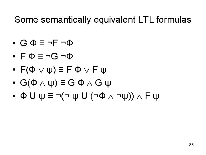
Semantically equivalent LTL formulas • Definition: Two LTL formulas Ф and ψ are semantically equivalent, writing as Ф ≡ ψ, if they are true for the same paths in each model. An LTL formula Ф is satisfied in a state s of a model if Ф is satisfied in every path starting at s. 82

Syntax of CTL* The CTL* formulas are divided into two classes: • state formulas, which are evaluated in states: Φ : : = p | T | (¬Φ) | (Φ Φ) | A[α] | E[α] where p is any atomic formula and any path formula; and • path formulas, which are evaluated along paths: α : : = Φ | (¬α) | (α U α) | (G α) | (F α) | (X α) where Φ is any state formula. 84

Semantics of CTL* (f 1 and f 2 are state formulas and g 1 and g 2 are path formulas) • • M, s ╞ p iff p ε L(s). M, s ╞ ¬ f 1 iff ¬(M, s ╞ f 1). M, s ╞ f 1 f 2 iff M, s ╞ f 1 and M, s ╞ f 2. M, s ╞ E g 1 iff there exists a path σ from s such that M, σ ╞ g 1. M, s ╞ A g 1 iff for every path σ starting from s, M, σ ╞ g 1. M, σ ╞ f 1 iff s is the first state of σ and M, s ╞ f 1. M, σ ╞ ¬ g 1 iff ¬(M, s ╞ g 1). M, σ ╞ g 1 g 2 iff M, σ ╞ g 1 and M, σ ╞ g 2. 85
 86")
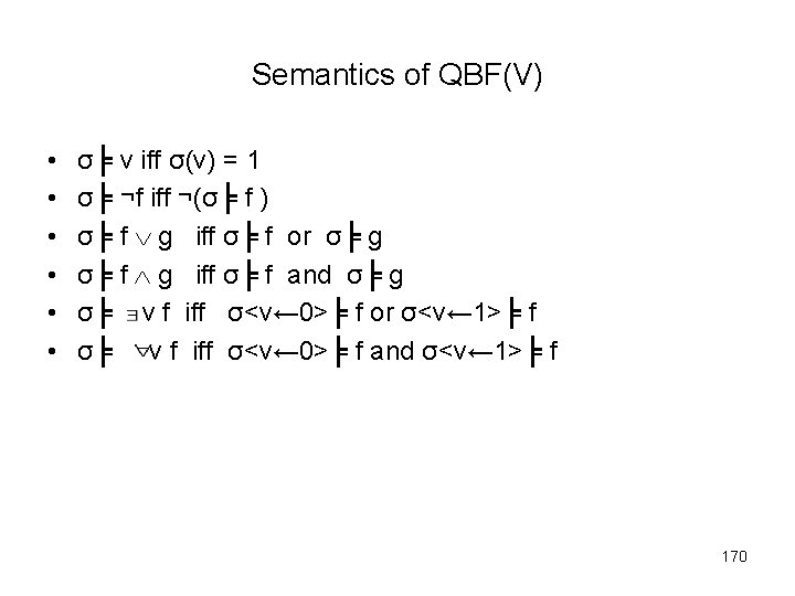
Semantics of QBF(V) 86
 (f 1 and f 2 are state formulas and g")
Semantics of CTL* (continued) (f 1 and f 2 are state formulas and g 1 and g 2 are path formulas) • • M, σ ╞ X g 1 iff M, σ1 ╞ g 1. M, σ ╞ F g 1 iff there exists a k ≥ 0 such that M, σk ╞ g 1. M, σ ╞ G g 1 iff for all k ≥ 0 , M, σk ╞ g 1. M, σ ╞ g 1 U g 2 iff there exists a k ≥ 0 such that M, σk ╞ g 2 and for all 0 ≤ j < k, M, σj ╞ g 1. 87

Theorem: • The set of operators ┴, ¬ and together with X, U and E are adequate for CTL*: any CTL* formula can be transformed into a semantically equivalent CTL formula which uses only those logical connectives. 88
 F f ≡ ¬┴")
Some interesting equivalences • • f g ≡ ¬(¬f ¬g) F f ≡ ¬┴ U f G f ≡ ¬F ¬f A(f) ≡ ¬E(¬f) 89

LTL and CTL as subsets of CTL* • Although the syntax of LTL does not include A and E, the semantic viewpoint of LTL is that we consider all paths. Therefore, the LTL formula α is equivalent to the CTL* formula A[α] • CTL is the fragment of CTL* in which we restrict the form of path formulas to α : : = (Φ U Φ) | (G Φ) | (F Φ) | (X Φ). 90

Example of in CTL but not in LTL: ψ1 = AG EF p • Whenever we have got to, we can always get back to a state in which p is true. This is useful, e. g. , in finding deadlocks in protocols. M s t ¬p p M’ s ¬p 91

Example of in CTL*, but neither in CTL nor in LTL: ψ2 = E[GF p] • Saying, there is a path with infinitely many p. 92

Example of in LTL but not in CTL: ψ3 = A[GF p → F q)] • Saying that if there are infinitely many p along the path, then there is an occurrence of q. • This is an interesting thing to be able to say; for example, many fairness constraints are of the form ‘infinitely often requested implies eventually acknowledged’. 93
 in")
Example of in LTL and CTL: ψ4 = AG (p → AF q) in CTL, or G (p → F q) in LTL • Saying, any p is eventually followed by a q. 94

Example • FG p and AF AG p are not semantically equivalent, since FG p is satisfied, whereas AF AG p is not satisfied, in the model p ¬p p 95
![weak until W • The formula A[p W q] is true in a state](http://slidetodoc.com/presentation_image_h/13b8c5681253cd7a843a0dde53fe06ec/image-96.jpg "weak until W • The formula A[p W q] is true in a state")
weak until W • The formula A[p W q] is true in a state if, along all paths from that state, p is true from the present state until the first state in which q is true, if any. In particular, if there is no q state on a path, then p needs to hold for all states of that path. 96
 • In LTL and CTL*, weak Until may be defined")
weak until W (continued) • In LTL and CTL*, weak Until may be defined in terms of the ordinary Until, as follows: p W q ≡ (p U q) G p • For CTL, we have: E[p W q] ≡ E[p U q] EG p A[p W q] ≡ ¬E[¬q U ¬(p q)] 97

A model-checking algorithm for CTL • INPUT: a Kripke structure M = (S, R, L) and a CTL formula Ф. • OUTPUT: the set of states of M which satisfy Ф. 98

function TRANSLATE • which takes as input an arbitrary CTL formula Ф and returns as output an equivalent CTL formula ψ whose only operators are among the set {┴, ¬, , AF, EU, EX}. 99
. • Next,")
The labelling algorithm • First, change Ф to the output of TRANSLATE(Ф). • Next, label the states of M with subformulas of Ф that are satisfied there, starting with the smallest formulas and working outwards towards Ф. 100
 • Suppose ψ is a subformula of Ф and states")
The labelling algorithm (continued) • Suppose ψ is a subformula of Ф and states satisfying all immediate subformulas of ψ have already been labelled (An immediate subformula of Ф is any maximal-length subformula other than Ф itself. ) We determine by a case analysis which states to label with ψ as follows. If ψ is: 101
 • ┴: then no states are labelled with ┴. •")
The labelling algorithm (continued) • ┴: then no states are labelled with ┴. • p: then label s with p if p ε L(s). • Ψ 1 Ψ 2: label s with Ψ 1 Ψ 2 if s is already labelled with Ψ 1 and with Ψ 2. • ¬Ψ 1: label s with ¬Ψ 1 if it is not already labelled with Ψ 1. • EX Ψ 1: label any state with EX Ψ 1 if one of its successors is labelled with Ψ 1. 102
 • AF ψ1: - If any state s is labeled")
The labelling algorithm (continued) • AF ψ1: - If any state s is labeled with ψ1, label it with AF ψ1. - Repeat: label any state with AF ψ1 if all successors states are labelled with AF ψ1, until there is no change. This step is illustrated in the figure of the next page. 103

The iteration step of the procedure for labelling states with subformulas of the form AFψ1. AF ψ1 AF ψ1 …until no change. AF ψ1 104
![The labelling algorithm (continued) • E[ψ1 U ψ2]: - If any state is labelled](http://slidetodoc.com/presentation_image_h/13b8c5681253cd7a843a0dde53fe06ec/image-105.jpg "The labelling algorithm (continued) • E[ψ1 U ψ2]: - If any state is labelled")
The labelling algorithm (continued) • E[ψ1 U ψ2]: - If any state is labelled with ψ2, label it with E[ψ1 U ψ2]. - Repeat: label any state with E[ψ1 U ψ2] if it is labelled with ψ1 and at least one of its successors is labelled with E[ψ1 U ψ2], until there is no change. This step is illustrated in the figure of the next page. 105

The iteration step of the procedure for labelling states with subformulas of the form E[ψ1 U ψ2] ψ1 ψ1 E[ψ1 U ψ2] … until no change. 106
), where")
The time complexity of the labelling algorithm • O(f. V. (V + E)), where f is the number of connectives in the formula, V is the number of states and E is the number of transitions. • The algorithm is linear in the size of the formula and quadratic in the size of the model. 107

A more efficient algorithm • Instead of using EX, EU and AF as the adequate set, we use EX, EU and EG instead. • For EX and EU we do as before. 108

For the case of EG, we have: • restrict the graph to states satisfying ψ, i. e. , delete all other states and their transitions. • find the maximal strongly connected components (SCC); there are maximal regions of the state space in which every state is linked with (= has a finite path to) every other one in that region. • use backwards breadth-first searching on the restricted graph to find any state that can reach an SCC. See the figure in the next page. 109

A better way of handling EG SCC ╞EG ψ SCC states satisfying ψ 110
),")
The time complexity of the more efficient labelling algorithm • O(f. (V + E)), where f is the number of connectives in the formula, V is the number of states and E is the number of transitions. • The algorithm is linear both in the size of the formula and the size of the model. 111

An example run of the labelling algorithm in our second model of mutual exclusion applied to the formula E[¬c 2 U c 1]. s 0 0: n 1 n 2 3: E[¬c 2 U c 1] s 1 0: t 1 n 2 2: E[¬c 2 U c 1] 0: n 1 t 2 s 3 0: c 1 n 2 1: E[¬c 2 U c 1] s 5 0: t 1 t 2 2: E[¬c 2 U c 1] s 4 0: c 1 t 2 1: E[¬c 2 U c 1] s 6 s 8 0: n 1 c 2 0: t 1 t 2 s 7 0: t 1 c 2 112
 /* determines the set")
The pseudo-code of the model checking algorithm function SAT (Φ) /* determines the set of states satisfying Φ */ begin case Φ is T: return S Φ is ┴: return Ø Φ is atomic: return {s ε S | Φ ε L(s)} Φ is Φ 1: return S – SAT(Φ 1) Φ is Φ 1 Φ 2: return SAT(Φ 1) ∩ SAT(Φ 2) Φ is EX Φ 1: return SATEX(Φ 1) Φ is AF Φ 1: return SATAF(Φ 1) Φ is EU Φ 1: return SATEU(Φ 1) end case end function 113
 /* determines the set of states satisfying EX Φ */ local")
The function SATEX(Φ) /* determines the set of states satisfying EX Φ */ local var X, Y begin X : = SAT(Φ); Y : = {s 0 ε S | (s 0, s 1) ε R for some s 1 ε X}; return Y end 114
 /* determines the set of states satisfying AF Φ */ local")
The function SATAF(Φ) /* determines the set of states satisfying AF Φ */ local var X, Y begin X : = S; Y : = SAT(Φ); repeat until X = Y begin X : = Y; Y : = Y U {s ε S | (s, s’) ε R for all s’ ε Y} end return Y end 115
 /* determines the set of states satisfying E[Φ U ψ)")
The function SATEU(Φ, ψ) /* determines the set of states satisfying E[Φ U ψ) */ local var W, X, Y begin W : = SAT(Φ); X : = S; Y : = SAT(ψ); repeat until X = Y begin X : = Y; Y : = Y U (W ∩ {s ε S | (s, s’) ε R for some s’ ε Y} end return Y end 116

fairness • Definition: Let C = {ψ1, ψ2, …, ψn} be a set of fairness constraints. A computation s 0 s 1 … is fair with respect to these fairness constraints if for each i, i = 1, …, n, there are infinitely many j, j = 0, 1, …, such that sj╞ ψi, that is, each ψi is true infinitely often along the path. 117

Model checking with fairness • Let AC and EC denote A and E restricted to fair paths. • Example: M, s 0╞ ACGФ iff Ф is true in every state along all fair paths; and similarly for ACF, ACU, etc. • It can be shown that ECG, ECU, and ECX form an adequate set. • We can also show EC[Ф U ψ] ≡ E[Ф U (ψ ECG T)] ECX Ф ≡ EX(Ф ECG T). 118
) Restrict the")
An algorithm for ECGФ • • with time complexity O(n. f. (V+E)) Restrict the graph to states satisfying Ф; of the resulting graph, we want to know from which states there is a fair path. Find the maximal strongly connected components (SCC) of the restricted graph; Remove an SCC if, for some ψi, it does not contain a state satisfying ψi. The resulting SCCs are the fair SCCs. Any state of the restricted graph that can reach one has a fair path from it. Use backwards breadth-first searching to find the states on the restricted graph that can reach a fair SCC. 119

Example: C = {ψ1, ψ2, ψ3} fair SCC ╞ EC GФ fair SCC ψ1 ψ2 ψ3 states satisfying Ф 120

Binary Decision Trees • Definition: A binary decision tree is a tree whose non-terminal nodes are labelled with boolean variables x, y, z, … and whose terminal nodes are labelled with either 0 or 1. Each nonterminal node has two edges, one dashed line and one solid line. x y 1 y 0 0 0 121
 • Definition: Let T be a finite binary decision tree.")
Binary Decision Trees (continued) • Definition: Let T be a finite binary decision tree. Then T determines a unique boolean function of the variables in non-terminal nodes, in the following way. Given an assignment of 0 s and 1 s to the boolean variables occurring in T, we start at the root of T and take the dashed line whenever the value at the current node is 0; otherwise, we travel along the solid line. The function value is the value of the terminal node we reach. 122
 = ¬(x + y) x y 1 y 0")
An example • f(x, y) = ¬(x + y) x y 1 y 0 0 0 123
 x y 1 y 0 124")
Some optimization techniques Binary Decision Diagrams (BDDs) x y 1 y 0 124
 x y 1 0 125")
Some optimization techniques (continued) x y 1 0 125

A BDD with duplicated sub. BDDs z x y 0 y y 1 126

after removal of one of the duplicate y-nodes z x y y 0 1 127

After removal of another duplicate y-nodes and then a redundant x-decision point z x y y 0 1 128

Three ways of reducing a BDD • Removal of a duplicate terminals. • Removal of a redundant tests. • Removal of duplicate non-terminals. 129
 • A directed acyclic graph (dag) is a directed graph")
Directed Acyclic Graphs (DAGs) • A directed acyclic graph (dag) is a directed graph that does not have any cycles. A node of a dag is initial if there are no edges pointing to that node. A node is terminal if there are no edges out of that node. 130
 • Definition: A binary decision diagram (BDD) is a finite")
Binary Decision Diagram (BDD) • Definition: A binary decision diagram (BDD) is a finite dag with a unique initial node, where all terminal nodes are labelled with 0 or 1 and all non-terminal nodes are labelled with a boolean variable. Each non-terminal node has exactly two edges from that node to others: one labelled 0 and one labelled 1 ( we represent them as a dashed line and a solid line, respectively). A BDD is said to be reduced if none of the earlier three optimization techniques can be applied (i. e. , no more reuctions are possible). 131
![Ordered Binary Decision Diagrams (OBDDs) • Definition: Let [x 1, …, xn] be an](http://slidetodoc.com/presentation_image_h/13b8c5681253cd7a843a0dde53fe06ec/image-132.jpg "Ordered Binary Decision Diagrams (OBDDs) • Definition: Let [x 1, …, xn] be an")
Ordered Binary Decision Diagrams (OBDDs) • Definition: Let [x 1, …, xn] be an ordered list of variables without duplications and let B be a BDD all of whose variables occur somewhere in the list. We say B has the ordering [x 1, …, xn] if all variables labels of B occur in that list and, for every occurrence of xj followed by xj along any path in B, we have i < j. • An ordered BDD (OBDD) is a BDD which has an ordering for some list of variables. 132
 and an OBDD (right) x x y x z")
Examples of a BDD (left) and an OBDD (right) x x y x z y 0 y x 1 y z 0 1 133

Reduced OBDDs as Canonical forms • Theorem: The reduced OBDD representing a given function f is unique. That is to say, let B 1 and B 2 be two reduced OBDDs with a compatible variable orderings. If B 1 and B 2 represent the same boolean function, then they have identical structure. 134

An OBDD for the even parity function for four bits x y y z z w w 1 0 135
. (z + w). (u + v) with variable")
The OBDD for (x + y). (z + w). (u + v) with variable ordering [x, y, z, w, u, v] x y z w u v 0 1 136
. (z + w). (u + v) with variable")
The OBDD for (x + y). (z + w). (u + v) with variable ordering [x, z, u, y, w, v] x z u y y u u y w w v 0 1 137

The importance of canonical representation • • • Absence of redundant variables. Test for semantic equivalence. Test for validity. Test for implication. Test for satisfiability. 138

The algorithm reduce in general terms • If the ordering of B is [x 1, x 2, …, xl], then B has at most l +1 layers. The algorithm reduce now traverses B layers in a bottom-up fashion (beginning with the terminal nodes). In traversing B, it assigns an integer label id(n) to each node n of B, in such a way that sub. OBDDs with root nodes n and m denote the same boolean function if, and only if, id(n) equals id(m). 139

The algorithm reduce • Definition: Given a non-terminal node n in a BDD, we define lo(n) to be the node pointed to via the dashed line from n. Dually, hi(n) is the node pointed to via the solid line from n. • Let us assume that reduce has already assigned integer labels to all nodes of a layer > i (i. e. , all terminal nodes and xj-nodes with j > i). We describe how nodes of layer i (i. e. , xi-nodes) are being handled as follows. 140
 Given an xi-node n, there are three ways in which")
The algorithm reduce (continued) Given an xi-node n, there are three ways in which it may get its label: • If the label id(lo(n)) is the same as id(hi(n)), then we set id(n) to be that label • If there is another node m such that n and m have the same variable xi, and id(lo(n)) = id(lo(m)) and id(hi(n)) = id(hi(m)), then we set id(n) to be id(m). • Otherwise, we set id(n) to the next unused integer label. 141

An example execution of the algorithm reduce #4 #4 x 1 #2 #3 x 2 #0 x 2 #2 x 3 #2 #2 x 3 0 #3 1 0 #1 #0 1 x 1 #0 0 1 #1 #1 142

The algorithm apply in general terms • Given OBDDs Bf and Bg for boolean formulas f and g, the call apply (op, Bf, Bg) computes the reduced OBDD of the boolean formula f op g, where op denotes any function from {0, 1} X {0, 1} to {0, 1}. 143

The algorithm apply The algorithm operates recursively on the structure of the two OBDDs: • Let v be the variable highest in the ordering (= leftmost in the list) which occurs in Bf or Bg. • Split the problem into subproblems for v being 0 and v being 1 and solve recursively; • At the leaves, apply the boolean operation op directly. 144

restrictions of f • Definition: Let f be a boolean formula and x a variable. We denote by f[0/x] the boolean formula obtained by replacing all occurrences of x in f by 0. The formula f[1/x] is defined similarly. The f[0/x] and f[1/x] are called restrictions of f. 145

Shannon expansion • Lemma: For all boolean formulas f and all boolean variables x (even those not occurring in f) we have f ≡ ¬x. f[0/x] + x. f[1/x]. • The function apply is based on the above lemma for f op g: f op g ≡ ¬xi. (f[0/xi] op g[0/xi]) + xi. (f[1/xi] op g[1/xi]). 146

The algorithm restrict in general terms • Given an OBDD Bf representing a boolean formula f, the call restrict (0, x, Bf) computes the reduced OBDD representing f[0/x] using the same variable ordering as B f. 147
 works as follows. For each")
The algorithm restrict • The algorithm restrict(0, x, Bf) works as follows. For each node n labelled with x, incoming edges are redirected to lo(n) and n is removed. Then we call reduce on the resulting OBDD. The call restrict(1, x, Bf) proceeds similarly, only we now redirect incoming edges to hi(n). 148
 B Output OBDD reduced B Time")
Time complexity Algorithm reduce apply restrict Input OBDD(s) B Output OBDD reduced B Time complexity O(|B|. Log |B|) Bf, Bg (reduced) Bf op g (reduced) O(|Bf|. |Bg|) Bf (reduced) Bf[0/x] or Bf[1/x] (reduced) O(|Bf|. Log |Bf|) 149

Symbolic Model Checking • Model checking using OBDDs is called symbolic model checking. • The term emphasizes that individual states are not represented; rather, sets of states are represented symbolically, namely, those which satisfy the formula being checked. 150

Representing subsets of the set of states • Let S be a finite set of states. The task is to represent the various subsets of S as OBDDs. • The way to do this in general is to assign to each element s ε S a unique vector of boolean values (v 1, v 2, …, vn), each vi ε {0, 1}. Then, we represent a subset T by the boolean function f. T which maps (v 1, v 2, …, vn) onto 1 if s ε T and maps it onto 0 otherwise. • Note that 2 n-1 < |S| ≤ 2 n. • The function f. T : {0, 1}n → {0, 1} which tells us, for each s, represented by (v 1, v 2, …, vn), whether it is in the set T or not, is called the characteristic function of T. 151
 • • • S =")
An example of a Kripke structure (S, R, L) • • • S = {s 0, s 1, s 2} R = {(s 0, s 1), (s 1, s 2), (s 2, s 0), (s 2, s 2)} L(s 0) = {x 1} L(s 1) = {x 2} s 0 x 1 s 1 x 2 L(s 2) = Ø s 2 152

Representation of subsets of states of the previous example set of states representation by boolean values Ø representation by boolean function 0 {s 0} (1, 0) x 1. ¬x 2 {s 1} (0, 1) ¬x 1. x 2 {s 2} (0, 0) ¬x 1. ¬x 2 {s 0, s 1} (1, 0), (0, 1) x 1. ¬x 2 + ¬x 1. x 2 {s 0, s 2} (1, 0), (0, 0) x 1. ¬x 2 + ¬x 1. ¬x 2 {s 1, s 2} (0, 1), (00) ¬x 1. x 2 + ¬x 1. ¬x 2 {s 0, s 1, s 2} (1, 0), (0, 1), (00) x 1. ¬x 2 + ¬x 1. ¬x 2 153

Two OBDDs for the set {s 0, s 1} of previous example x 1 x 2 0 1 x 1 + x 2 x 1 x 2 0 1 x 1. ¬x 2 + ¬x 1. x 2 154

Representing transition relations • The transition relation R of a Kripke structure (S, R, L) is a subset of S × S. So, as a subset of a given set, it may be represented as an OBDD. • Thus, a transition (s, s’) ε R can be represented by a pair of boolean vectors (v 1, …, vn), (v’ 1, …, v’n), where (v 1, …, vn) represents s and (v’ 1, …, v’n) represents s’. 155

The boolean function representation for the transition relation of the previous example • f. R = x 1. ¬x 2. ¬x’ 1. x’ 2 + ¬x 1. x 2. ¬x’ 1. ¬x’ 2 + ¬x 1. ¬x 2. ¬x’ 1. ¬x’ 2 156

The truth table for the transition relation of the previous example with ordering [x 1, x 2, x’ 1, x’ 2] x 1 x 2 x’ 1 x’ 2 R 0 0 1 0 0 1 1 _ 0 1 0 0 1 1 1 _ 1 0 0 1 1 1 0 0 1 1 _ 1 1 0 0 _ 1 1 0 1 _ 1 1 1 0 _ 1 1 _ 157

The truth table for the transition relation of the previous example with ordering [x 1, x’ 1, x 2, x’ 2] x 1 x’ 1 x 2 x’ 2 R 0 0 1 0 0 1 1 0 0 1 1 0 _ 0 0 1 1 1 _ 1 0 0 1 1 1 0 1 0 1 1 _ _ 1 1 0 0 0 1 1 0 1 _ 1 1 1 0 _ 1 1 _ 158

An OBDD for the transition relation of the previous example. x 1 X’ 1 x 2 X’ 2 0 1 159
 be an arbitrary finite Kripke")
Fixpoint Representation • Let M = (S, R, L) be an arbitrary finite Kripke structure. The set P(S) of all subsets of S form a lattice under the set inclusion ordering. • Each element S’ of the lattice can be thought as a predicate on S, where the predicate is viewed as being true for exactly the states in S’. • A function that maps P(S) to P(S) is called a predicate transformer. 160
 → P(S) be a predicate transformer; then: •")
Fixpoint theory Let t : P(S) → P(S) be a predicate transformer; then: • t is monotonic provided that P Q implies t(P) t(Q); • t is U-continuous provided P 1 P 2 … implies t(Ui Pi) = Ui t(Pi); • t is ∩-continuous provided P 1 P 2 … implies t(∩i Pi) = ∩i t(Pi). 161
 • Let t i (Z) denote i applications of t to")
Fixpoint theory (continued) • Let t i (Z) denote i applications of t to Z. • According to Tarski, any monotonic predicate transformer t on P(S) always has a least fixpoint μZ. t(Z), and a greatest fixpoint ע Z. t(Z) where μZ. t(Z) = ∩{Z | t(Z) Z} and ע Z. t(Z) = U{Z | t(Z) Z}. • Additionally, if t is U-continuous μZ. t(Z) = Ui t i (False) and if t is ∩-continuous ע Z. t(Z) = ∩i t i (True). 162

Some properties • Lemma 1: If S is finite and t is monotonic, then t is also U-continuous and ∩-continuous. • Lemma 2: If t is monotonic, then for every i, t i (False) and t i (True) t i+1 (True). • Lemma 3: If t is monotonic and S is finite, then there is an integer i 0 such that for every j ≥ i 0, t j (False) = t i 0 (False). Similarly, there is some j 0 such that for every j ≥ j 0, t j (True) = t j 0 (True). • Lemma 4: If t is monotonic and S is finite, then there is an integer i 0 such that μZ. t(Z) = t i 0 (False). Similarly, there is some j 0 such that ע Z. t(Z) = t j 0 (True). t i+1 (False) 163
 : Predicate Q")
Procedure for computing least fixpoint • function Lfp(Tau : Predicate. Transformer) : Predicate Q : = False; Q’ : = Tau(Q); while (Q ≠ Q’) do Q : = Q’; Q’ : = Tau(Q’); end while; return(Q); end function 164
 : Predicate Q")
Procedure for computing greatest fixpoint • function Gfp(Tau : Predicate. Transformer) : Predicate Q : = True; Q’ : = Tau(Q); while (Q ≠ Q’) do Q : = Q’; Q’ : = Tau(Q’); end while; return(Q); end function 165

CTL operators as greatest or least fixpoints • If we identify each CTL formula f with the predicate {s | M, s╞ f}, then each of the basic CTL operators may be characterized as a least or greatest fixpoint of an appropriate predicate transformer as follows: • • • AF f 1 = μZ. f 1 AX Z EF f 1 = μZ. f 1 EX Z AG f 1 = ע Z. f 1 AX Z EG f 1 = ע Z. f 1 EX Z A[f 1 U f 2] = μZ. f 2 (f 1 AX Z) E[f 1 U f 2] = μZ. f 2 (f 1 EX Z) 166
![Sequence of approximations for E[p U q] p q t 1 (False) Kripke structure](http://slidetodoc.com/presentation_image_h/13b8c5681253cd7a843a0dde53fe06ec/image-167.jpg "Sequence of approximations for E[p U q] p q t 1 (False) Kripke structure")
Sequence of approximations for E[p U q] p q t 1 (False) Kripke structure s 0 p t 2 (False) q s 0 p p p q s 0 p t 3 (False) 167
 • Given a set V = {v 0, …, vn-1}")
Quantified Boolean Formulas (QBF) • Given a set V = {v 0, …, vn-1} of propositional variables, QBF(V) is the smallest set of formulas such that: • Every variable in V is a formula. • If f and g are formulas, then ¬ f, f g are formulas. • If f and g are formulas, then v f and v f are formulas. 168
 is a function σ : V")
Truth Assignment • A truth assignment for QBF(V) is a function σ : V → {0, 1}. • We will use the notation σ<v←a> for the truth assignment defined by σ<v←a>(w) = a, if v = w; σ<v←a>(w) = σ(w), otherwise. 169
![OBDDs for Quantification operators • • x f = f[0/x] f[1/x] 171](http://slidetodoc.com/presentation_image_h/13b8c5681253cd7a843a0dde53fe06ec/image-171.jpg "OBDDs for Quantification operators • • x f = f[0/x] f[1/x] 171")
OBDDs for Quantification operators • • x f = f[0/x] f[1/x] 171

The Symbolic Model-Checking Algorithm • The symbolic model-checking algorithm is implemented by a procedure Check that takes the CTL formula to be checked as its argument and returns an OBDD that represents exactly those states of the system that satisfy the formula. • We define check inductively over the structure of CTL formulas. 172
 • If f = f 1 f 2 or")
The Symbolic Model-Checking Algorithm (continued) • If f = f 1 f 2 or f = ¬ f 1, then Check(f) is obtained by using the function Apply described before. • Formulas of the form EX f, E[f U g], and EG f are handled by the procedures Check(EX f) = Check. EX(Check(f)) Check(E[f U g]) = Check. EU(Check(f), Check(g)) Check(EG f) = Check. EG(Check(f)) 173
![The Symbolic Model-Checking Algorithm (continued) • Check. EX(f(v)) = v’ [ f(v’) R(v, v’)]](http://slidetodoc.com/presentation_image_h/13b8c5681253cd7a843a0dde53fe06ec/image-174.jpg "The Symbolic Model-Checking Algorithm (continued) • Check. EX(f(v)) = v’ [ f(v’) R(v, v’)]")
The Symbolic Model-Checking Algorithm (continued) • Check. EX(f(v)) = v’ [ f(v’) R(v, v’)] using the operations of QBF. • E[f 1 U f 2] = μZ. f 2 (f 1 EX Z) using the function Lfp. • EG f 1 = ע Z. f 1 EX Z using the function Gfp. 174
- Slides: 174