Chapter 2 Matrices 2 1 Operations with Matrices
- Slides: 89

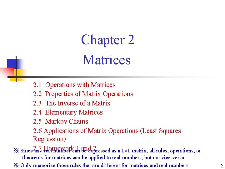
Chapter 2 Matrices 2. 1 Operations with Matrices 2. 2 Properties of Matrix Operations 2. 3 The Inverse of a Matrix 2. 4 Elementary Matrices 2. 5 Markov Chains 2. 6 Applications of Matrix Operations (Least Squares Regression) 2. 7 Homework 1 and 2 ※ Since any real number can be expressed as a 1 1 matrix, all rules, operations, or theorems for matrices can be applied to real numbers, but not vice versa ※ Only memorize those rules that are different for matrices and real numbers 2.

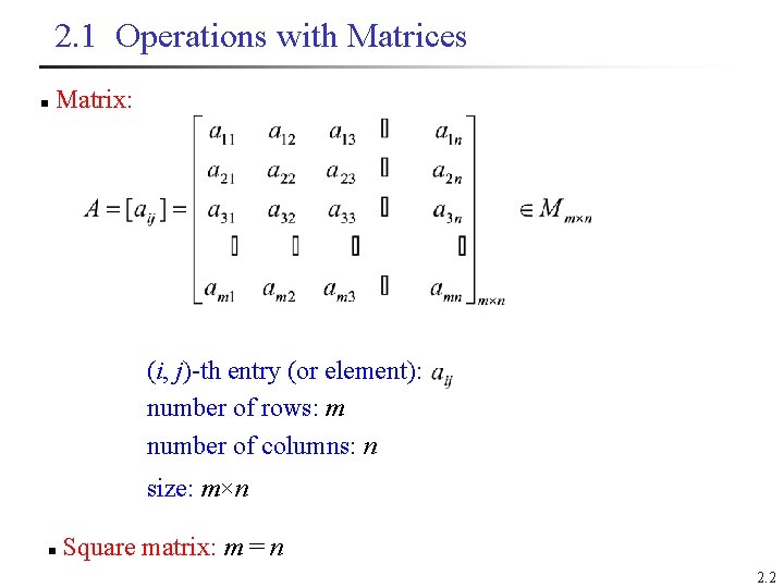
2. 1 Operations with Matrices Matrix: n (i, j)-th entry (or element): number of rows: m number of columns: n size: m×n Square matrix: m = n n 2. 2

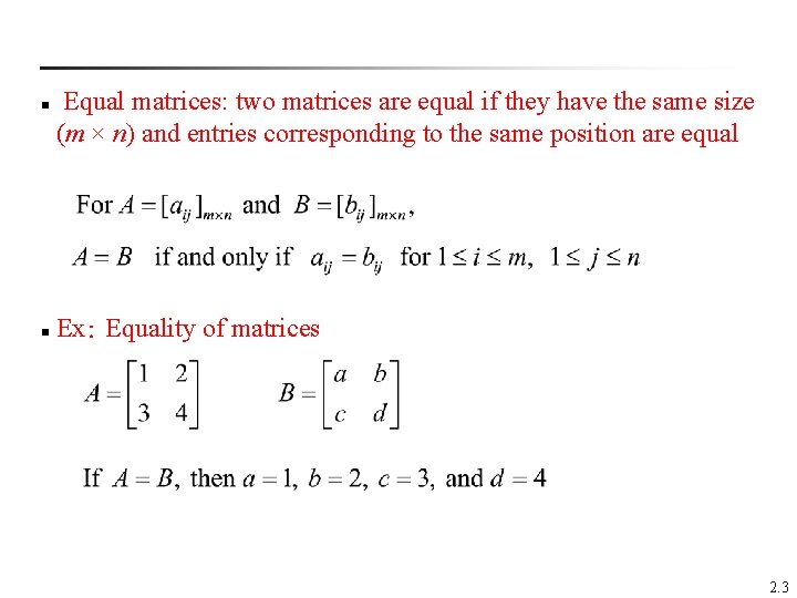
n Equal matrices: two matrices are equal if they have the same size (m × n) and entries corresponding to the same position are equal Ex: Equality of matrices n 2. 3

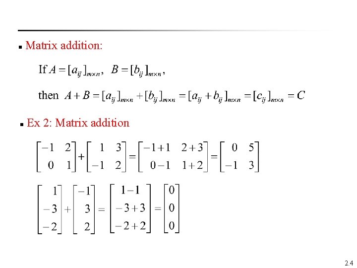
Matrix addition: n Ex 2: Matrix addition n 2. 4

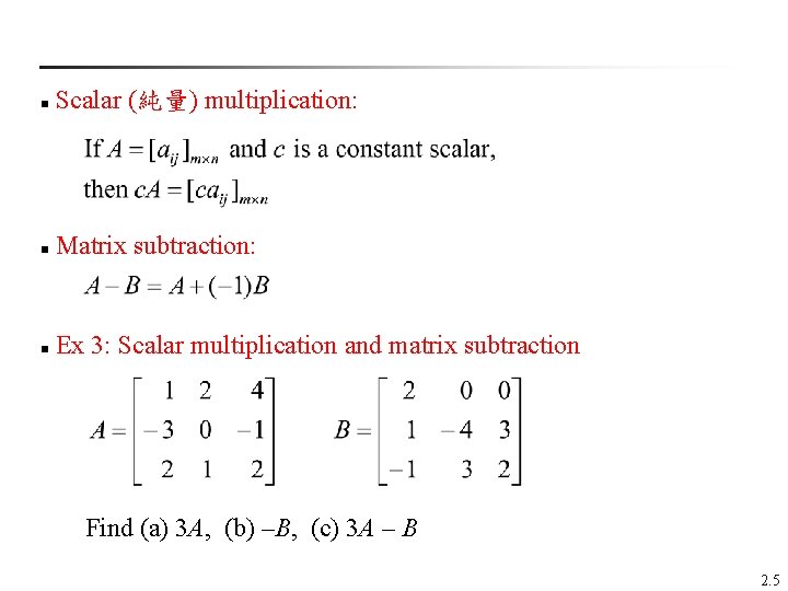
Scalar (純量) multiplication: n Matrix subtraction: n Ex 3: Scalar multiplication and matrix subtraction n Find (a) 3 A, (b) –B, (c) 3 A – B 2. 5

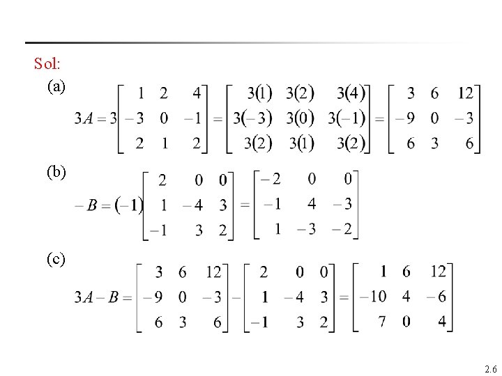
Sol: (a) (b) (c) 2. 6

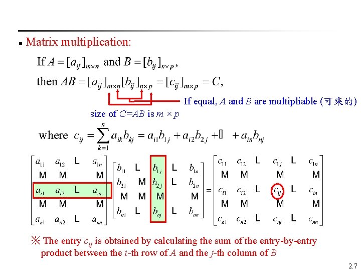
Matrix multiplication: n If equal, A and B are multipliable (可乘的) size of C=AB is m × p where ※ The entry cij is obtained by calculating the sum of the entry-by-entry product between the i-th row of A and the j-th column of B 2. 7

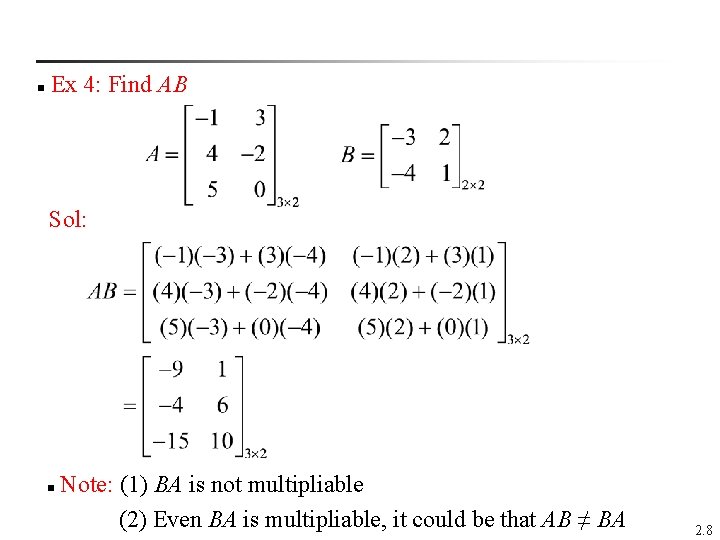
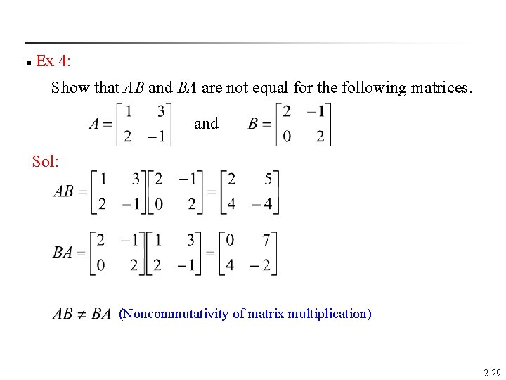
Ex 4: Find AB n Sol: Note: (1) BA is not multipliable (2) Even BA is multipliable, it could be that AB ≠ BA n 2. 8

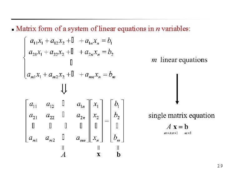
Matrix form of a system of linear equations in n variables: n x = = = A b 2. 9

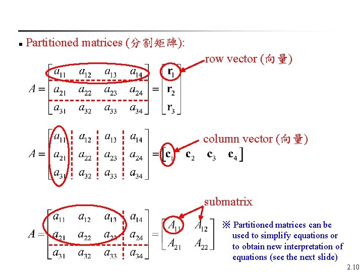
Partitioned matrices (分割矩陣): n row vector (向量) column vector (向量) submatrix ※ Partitioned matrices can be used to simplify equations or to obtain new interpretation of equations (see the next slide) 2. 10

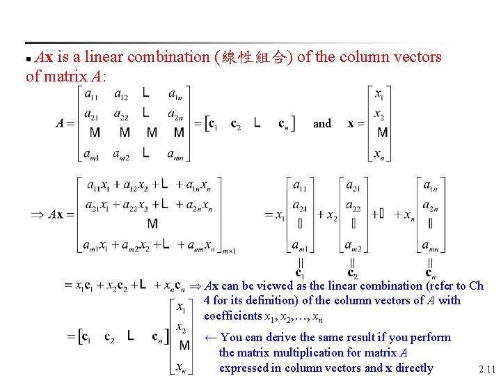
Ax is a linear combination (線性組合) of the column vectors of matrix A: n and = = = Ax can be viewed as the linear combination (refer to Ch 4 for its definition) of the column vectors of A with coefficients x 1, x 2, …, xn ← You can derive the same result if you perform the matrix multiplication for matrix A expressed in column vectors and x directly 2. 11

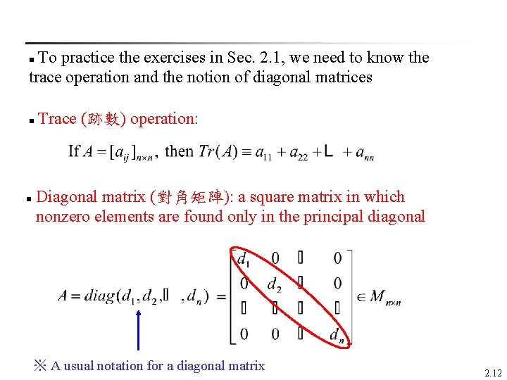
To practice the exercises in Sec. 2. 1, we need to know the trace operation and the notion of diagonal matrices n Trace (跡數) operation: n n Diagonal matrix (對角矩陣): a square matrix in which nonzero elements are found only in the principal diagonal ※ A usual notation for a diagonal matrix 2. 12

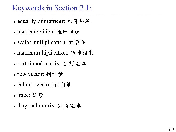
Keywords in Section 2. 1: n equality of matrices: 相等矩陣 n matrix addition: 矩陣相加 n scalar multiplication: 純量積 n matrix multiplication: 矩陣相乘 n partitioned matrix: 分割矩陣 n row vector: 列向量 n column vector: 行向量 n trace: 跡數 n diagonal matrix: 對角矩陣 2. 13

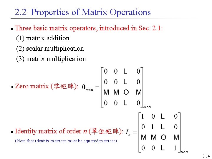
2. 2 Properties of Matrix Operations Three basic matrix operators, introduced in Sec. 2. 1: (1) matrix addition (2) scalar multiplication (3) matrix multiplication n Zero matrix (零矩陣): n n Identity matrix of order n (單位矩陣): (Note that identity matrices must be squared matrices) 2. 14

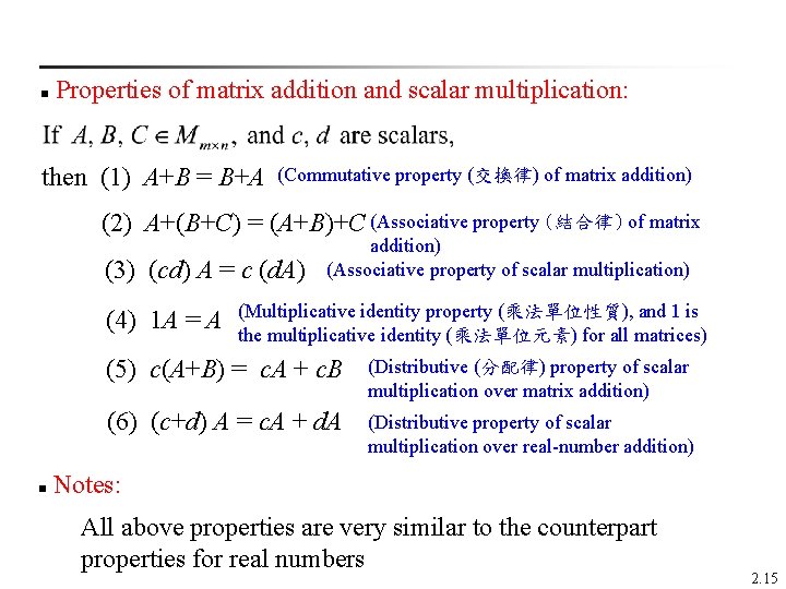
Properties of matrix addition and scalar multiplication: n then (1) A+B = B+A (Commutative property (交換律) of matrix addition) (2) A+(B+C) = (A+B)+C (Associative property (結合律) of matrix (3) (cd) A = c (d. A) (4) 1 A = A addition) (Associative property of scalar multiplication) (Multiplicative identity property (乘法單位性質), and 1 is the multiplicative identity (乘法單位元素) for all matrices) (5) c(A+B) = c. A + c. B (Distributive (分配律) property of scalar multiplication over matrix addition) (6) (c+d) A = c. A + d. A (Distributive property of scalar multiplication over real-number addition) Notes: n All above properties are very similar to the counterpart properties for real numbers 2. 15

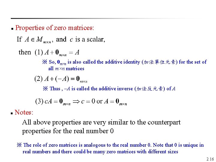
Properties of zero matrices: n ※ So, 0 m×n is also called the additive identity (加法單位元素) for the set of all m×n matrices ※ Thus , –A is called the additive inverse (加法反元素) of A Notes: All above properties are very similar to the counterpart properties for the real number 0 n ※ The role of zero matrices is analogous to the real number 0. Note that 0 is unique in real numbers and there could be many zero matrices with different sizes 2. 16

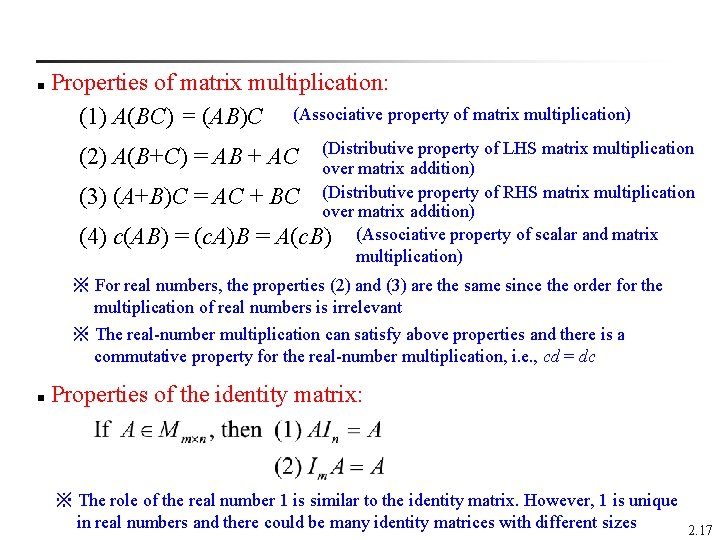
Properties of matrix multiplication: (1) A(BC) = (AB)C (Associative property of matrix multiplication) n (Distributive property of LHS matrix multiplication over matrix addition) (3) (A+B)C = AC + BC (Distributive property of RHS matrix multiplication over matrix addition) (4) c(AB) = (c. A)B = A(c. B) (Associative property of scalar and matrix multiplication) (2) A(B+C) = AB + AC ※ For real numbers, the properties (2) and (3) are the same since the order for the multiplication of real numbers is irrelevant ※ The real-number multiplication can satisfy above properties and there is a commutative property for the real-number multiplication, i. e. , cd = dc Properties of the identity matrix: n ※ The role of the real number 1 is similar to the identity matrix. However, 1 is unique in real numbers and there could be many identity matrices with different sizes 2. 17

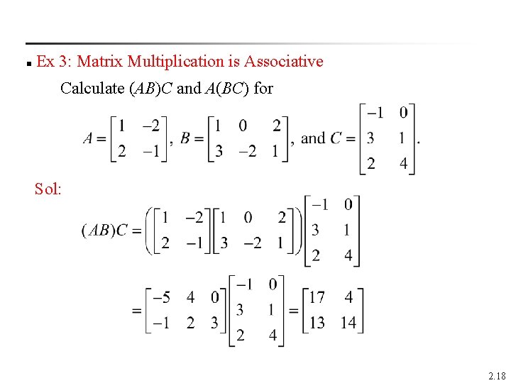
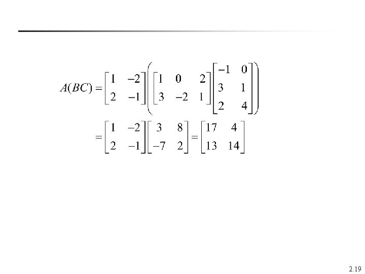
Ex 3: Matrix Multiplication is Associative n Calculate (AB)C and A(BC) for Sol: 2. 18

2. 19

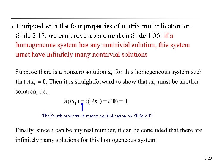
n Equipped with the four properties of matrix multiplication on Slide 2. 17, we can prove a statement on Slide 1. 35: if a homogeneous system has any nontrivial solution, this system must have infinitely many nontrivial solutions The fourth property of matrix multiplication on Slide 2. 17 2. 20

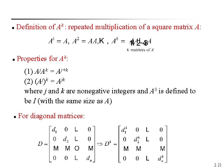
Definition of Ak : repeated multiplication of a square matrix A: n Properties for Ak: n (1) Aj. Ak = Aj+k (2) (Aj)k = Ajk where j and k are nonegative integers and A 0 is defined to be I (with the same size as A) For diagonal matrices: n 2. 21

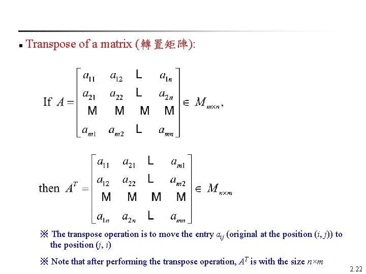
Transpose of a matrix (轉置矩陣): n ※ The transpose operation is to move the entry aij (original at the position (i, j)) to the position (j, i) ※ Note that after performing the transpose operation, AT is with the size n×m 2. 22

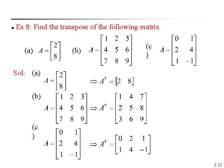
Ex 8: Find the transpose of the following matrix n (a) (b) (c ) Sol: (a) (b) (c ) 2. 23

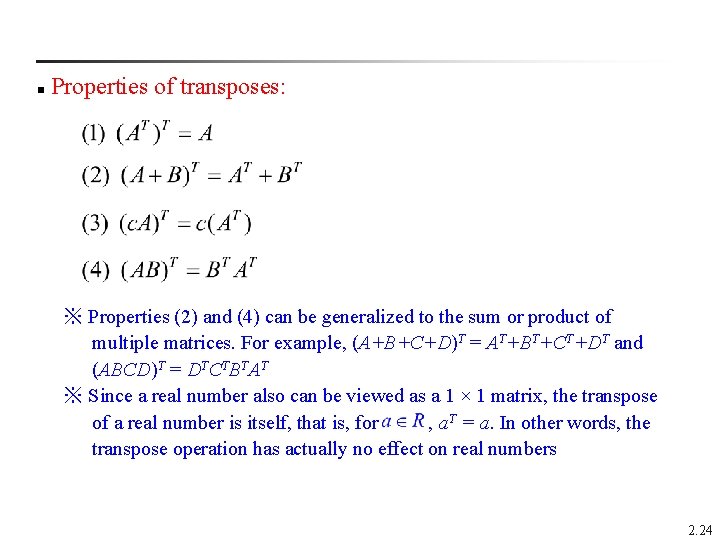
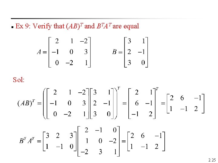
Properties of transposes: n ※ Properties (2) and (4) can be generalized to the sum or product of multiple matrices. For example, (A+B+C+D)T = AT+BT+CT+DT and (ABCD)T = DTCTBTAT ※ Since a real number also can be viewed as a 1 × 1 matrix, the transpose of a real number is itself, that is, for , a. T = a. In other words, the transpose operation has actually no effect on real numbers 2. 24

Ex 9: Verify that (AB)T and BTAT are equal n Sol: 2. 25

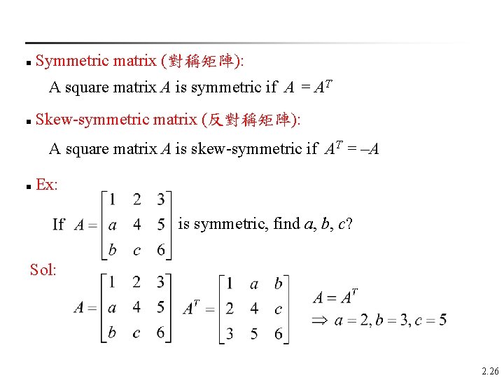
Symmetric matrix (對稱矩陣): n A square matrix A is symmetric if A = AT Skew-symmetric matrix (反對稱矩陣): n A square matrix A is skew-symmetric if AT = –A Ex: n is symmetric, find a, b, c? Sol: 2. 26

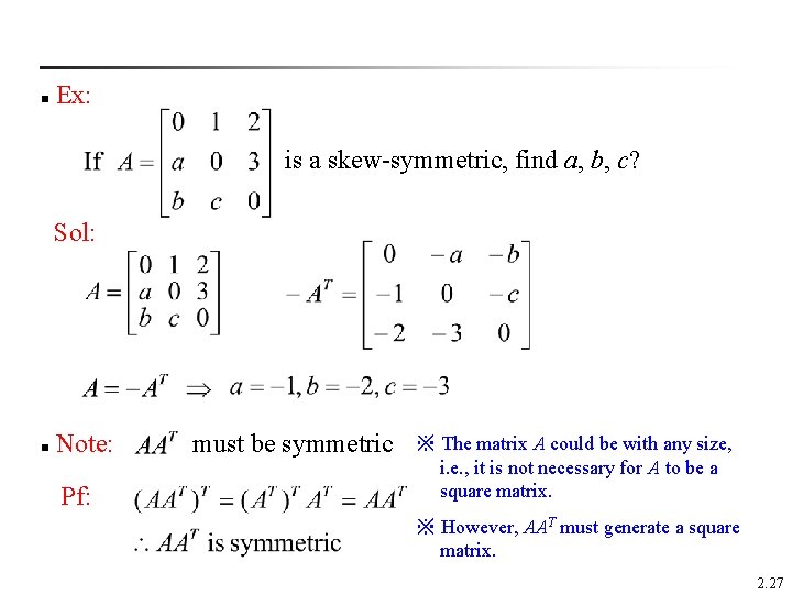
Ex: n is a skew-symmetric, find a, b, c? Sol: Note: n Pf: must be symmetric ※ The matrix A could be with any size, i. e. , it is not necessary for A to be a square matrix. ※ However, AAT must generate a square matrix. 2. 27

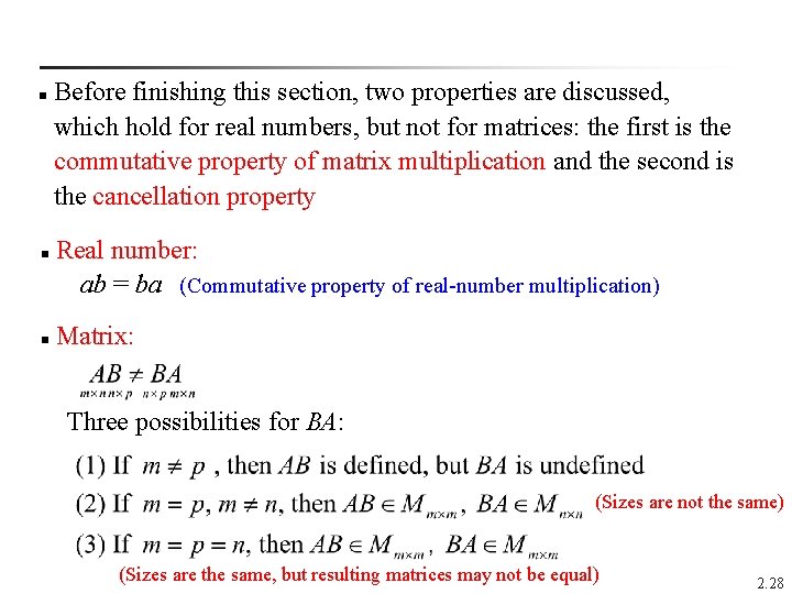
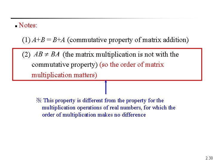
Before finishing this section, two properties are discussed, which hold for real numbers, but not for matrices: the first is the commutative property of matrix multiplication and the second is the cancellation property n Real number: ab = ba (Commutative property of real-number multiplication) n Matrix: n Three possibilities for BA: (Sizes are not the same) (Sizes are the same, but resulting matrices may not be equal) 2. 28

Ex 4: n Show that AB and BA are not equal for the following matrices. and Sol: (Noncommutativity of matrix multiplication) 2. 29

Notes: n (1) A+B = B+A (commutative property of matrix addition) (2) (the matrix multiplication is not with the commutative property) (so the order of matrix multiplication matters) ※ This property is different from the property for the multiplication operations of real numbers, for which the order of multiplication makes no difference 2. 30

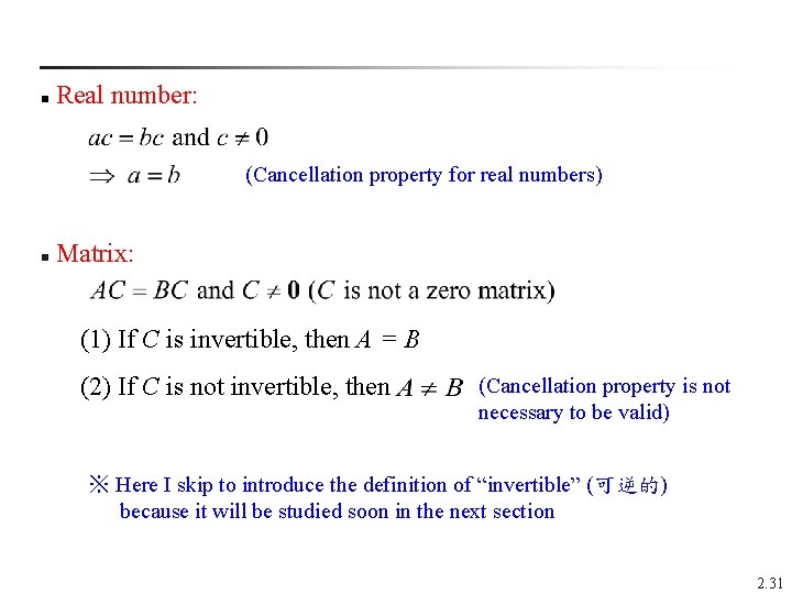
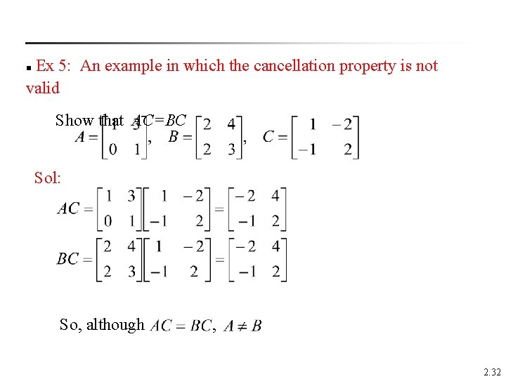
Real number: n (Cancellation property for real numbers) Matrix: n (1) If C is invertible, then A = B (2) If C is not invertible, then (Cancellation property is not necessary to be valid) ※ Here I skip to introduce the definition of “invertible” (可逆的) because it will be studied soon in the next section 2. 31

Ex 5: An example in which the cancellation property is not valid n Show that AC=BC Sol: So, although , 2. 32

Keywords in Section 2. 2: n zero matrix: 零矩陣 n identity matrix: 單位矩陣 n commutative property: 交換律 n associative property: 結合律 n distributive property: 分配律 n cancellation law: 消去法則 n transpose matrix: 轉置矩陣 n symmetric matrix: 對稱矩陣 n skew-symmetric matrix: 反對稱矩陣 2. 33

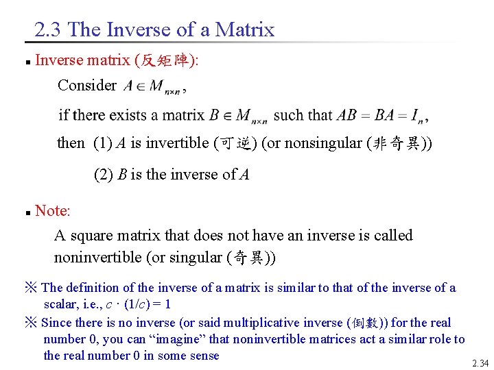
2. 3 The Inverse of a Matrix Inverse matrix (反矩陣): n Consider , then (1) A is invertible (可逆) (or nonsingular (非奇異)) (2) B is the inverse of A Note: A square matrix that does not have an inverse is called noninvertible (or singular (奇異)) n ※ The definition of the inverse of a matrix is similar to that of the inverse of a scalar, i. e. , c · (1/c) = 1 ※ Since there is no inverse (or said multiplicative inverse (倒數)) for the real number 0, you can “imagine” that noninvertible matrices act a similar role to the real number 0 in some sense 2. 34

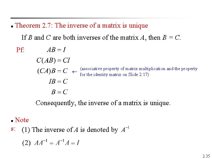
Theorem 2. 7: The inverse of a matrix is unique n If B and C are both inverses of the matrix A, then B = C. Pf: (associative property of matrix multiplication and the property for the identity matrix on Slide 2. 17) Consequently, the inverse of a matrix is unique. Note s: (1) The inverse of A is denoted by n 2. 35

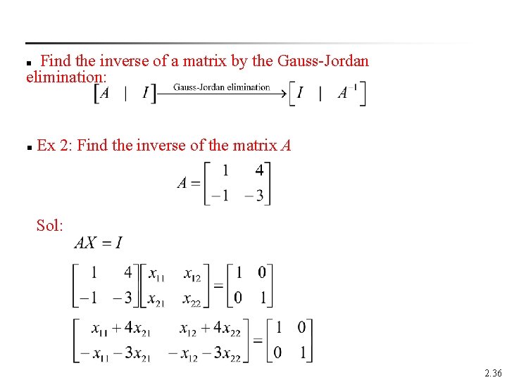
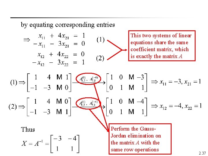
Find the inverse of a matrix by the Gauss-Jordan elimination: n Ex 2: Find the inverse of the matrix A n Sol: 2. 36

by equating corresponding entries This two systems of linear equations share the same coefficient matrix, which is exactly the matrix A Thus Perform the Gauss. Jordan elimination on the matrix A with the same row operations 2. 37

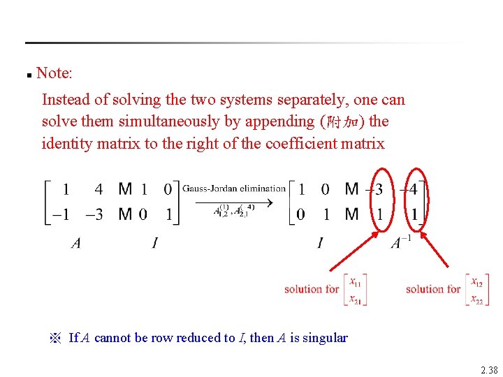
Note: n Instead of solving the two systems separately, one can solve them simultaneously by appending (附加) the identity matrix to the right of the coefficient matrix ※ If A cannot be row reduced to I, then A is singular 2. 38

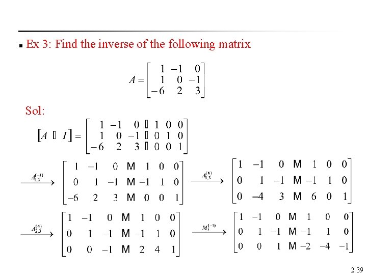
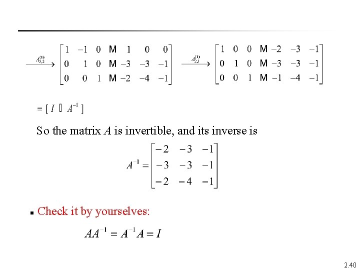
Ex 3: Find the inverse of the following matrix n Sol: 2. 39

So the matrix A is invertible, and its inverse is n Check it by yourselves: 2. 40

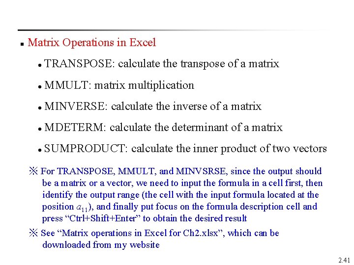
n Matrix Operations in Excel TRANSPOSE: calculate the transpose of a matrix l MMULT: matrix multiplication l MINVERSE: calculate the inverse of a matrix l MDETERM: calculate the determinant of a matrix l SUMPRODUCT: calculate the inner product of two vectors l ※ For TRANSPOSE, MMULT, and MINVSRSE, since the output should be a matrix or a vector, we need to input the formula in a cell first, then identify the output range (the cell with the input formula located at the position a 11), and finally put focus on the formula description cell and press “Ctrl+Shift+Enter” to obtain the desired result ※ See “Matrix operations in Excel for Ch 2. xlsx”, which can be downloaded from my website 2. 41

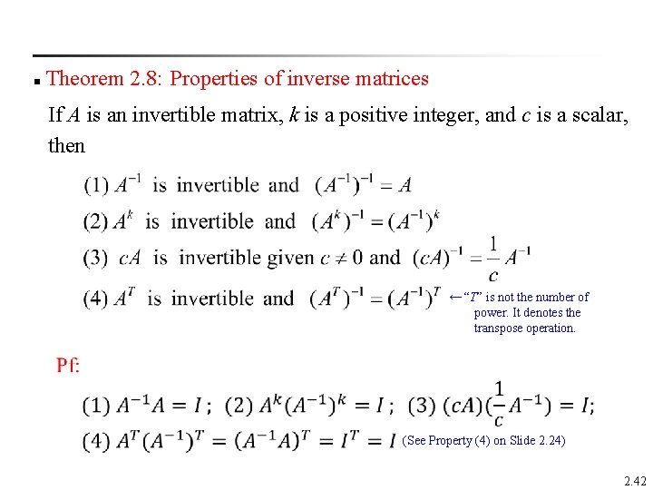
Theorem 2. 8: Properties of inverse matrices n If A is an invertible matrix, k is a positive integer, and c is a scalar, then ← “T” is not the number of power. It denotes the transpose operation. n (See Property (4) on Slide 2. 24) 2. 42

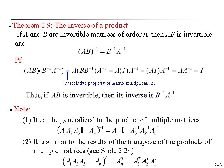
Theorem 2. 9: The inverse of a product If A and B are invertible matrices of order n, then AB is invertible and n Pf: (associative property of matrix multiplication) Note: (1) It can be generalized to the product of multiple matrices n (2) It is similar to the results of the transpose of the products of multiple matrices (see Slide 2. 24) 2. 43

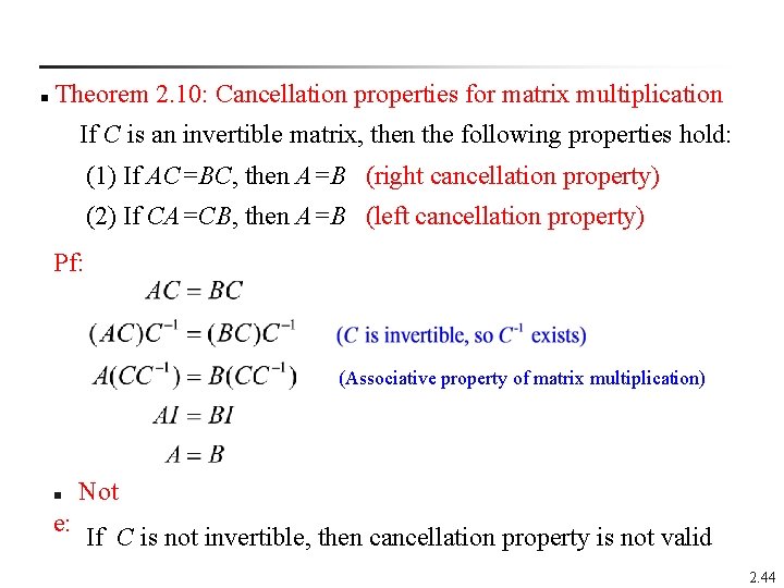
Theorem 2. 10: Cancellation properties for matrix multiplication n If C is an invertible matrix, then the following properties hold: (1) If AC=BC, then A=B (right cancellation property) (2) If CA=CB, then A=B (left cancellation property) Pf: (Associative property of matrix multiplication) Not e: If C is not invertible, then cancellation property is not valid n 2. 44

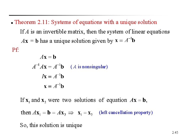
Theorem 2. 11: Systems of equations with a unique solution n If A is an invertible matrix, then the system of linear equations Ax = b has a unique solution given by Pf: ( A is nonsingular) (left cancellation property) So, this solution is unique 2. 45

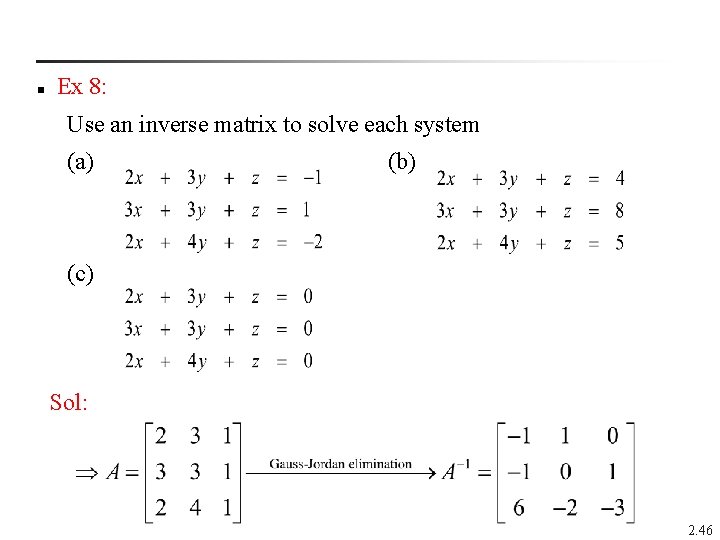
n Ex 8: Use an inverse matrix to solve each system (a) (b) (c) Sol: 2. 46

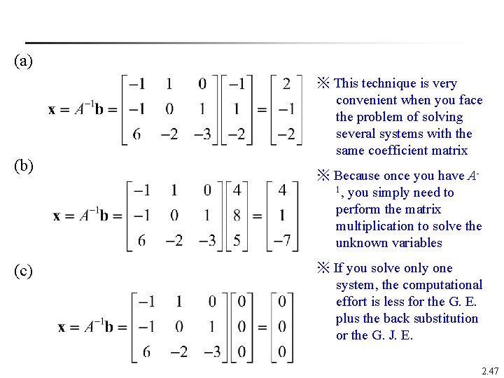
(a) (b) (c) ※ This technique is very convenient when you face the problem of solving several systems with the same coefficient matrix ※ Because once you have A 1, you simply need to perform the matrix multiplication to solve the unknown variables ※ If you solve only one system, the computational effort is less for the G. E. plus the back substitution or the G. J. E. 2. 47

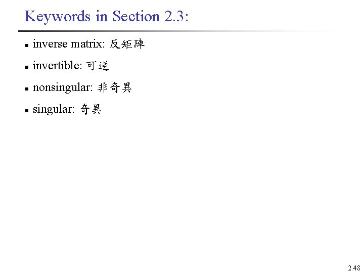
Keywords in Section 2. 3: n inverse matrix: 反矩陣 n invertible: 可逆 n nonsingular: 非奇異 n singular: 奇異 2. 48

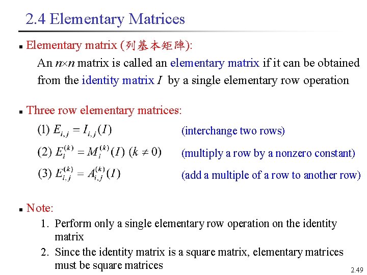
2. 4 Elementary Matrices Elementary matrix (列基本矩陣): An n n matrix is called an elementary matrix if it can be obtained from the identity matrix I by a single elementary row operation n n Three row elementary matrices: (interchange two rows) (multiply a row by a nonzero constant) (add a multiple of a row to another row) n Note: 1. Perform only a single elementary row operation on the identity matrix 2. Since the identity matrix is a square matrix, elementary matrices must be square matrices 2. 49

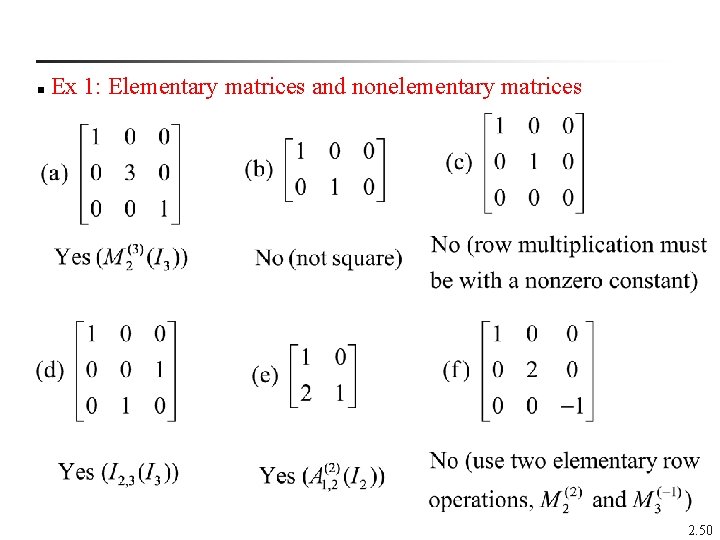
Ex 1: Elementary matrices and nonelementary matrices n 2. 50

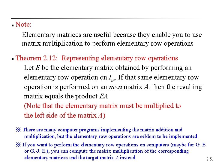
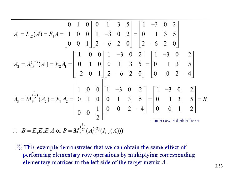
Note: Elementary matrices are useful because they enable you to use matrix multiplication to perform elementary row operations n Theorem 2. 12: Representing elementary row operations Let E be the elementary matrix obtained by performing an elementary row operation on Im. If that same elementary row operation is performed on an m n matrix A, then the resulting matrix equals the product EA (Note that the elementary matrix must be multiplied to the left side of the matrix A) n ※ There are many computer programs implementing the matrix addition and multiplication, but the elementary row operations are seldom to be implemented ※ If you want to perform the elementary row operations on computers (maybe for G. E. or G. -J. E. ), you can compute the matrix multiplication of the corresponding elementary matrices and the target matrix A instead 2. 51

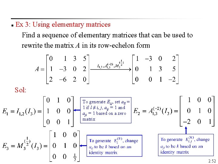
Ex 3: Using elementary matrices Find a sequence of elementary matrices that can be used to rewrite the matrix A in its row-echelon form n Sol: To generate Ei, j, set all = 1 if l ≠ i, j, aij = 1 and aji = 1 based on a zero matrix n n 2. 52

same row-echelon form ※ This example demonstrates that we can obtain the same effect of performing elementary row operations by multiplying corresponding elementary matrices to the left side of the target matrix A 2. 53

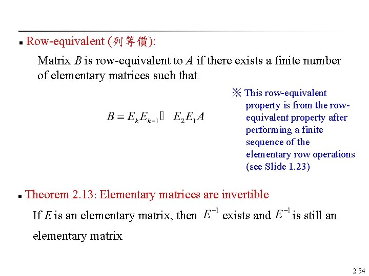
Row-equivalent (列等價): n Matrix B is row-equivalent to A if there exists a finite number of elementary matrices such that ※ This row-equivalent property is from the rowequivalent property after performing a finite sequence of the elementary row operations (see Slide 1. 23) Theorem 2. 13: Elementary matrices are invertible n If E is an elementary matrix, then exists and is still an elementary matrix 2. 54

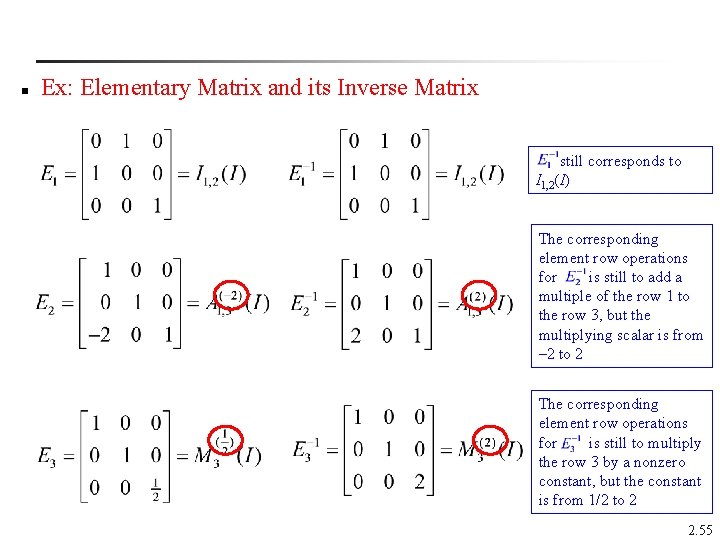
n Ex: Elementary Matrix and its Inverse Matrix still corresponds to I 1, 2(I) The corresponding element row operations for is still to add a multiple of the row 1 to the row 3, but the multiplying scalar is from – 2 to 2 The corresponding element row operations for is still to multiply the row 3 by a nonzero constant, but the constant is from 1/2 to 2 2. 55

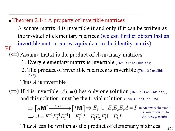
Theorem 2. 14: A property of invertible matrices A square matrix A is invertible if and only if it can be written as the product of elementary matrices (we can further obtain that an invertible matrix is row-equivalent to the identity matrix) Pf: Assume that A is the product of elementary matrices 1. Every elementary matrix is invertible (Thm. 2. 13 on Slide 2. 53) 2. The product of invertible matrices is invertible (Thm. 2. 9 on Slide n 2. 43) Thus A is invertible If A is invertible, has only one solution (Thm. 2. 11 on Slide 2. 45), and this solution must be the trivial solution (Thm. 1. 1 on Slide 1. 35). An invertible matrix is row-equivalent to the identity matrix Thus A can be written as the product of elementary matrices 2. 56

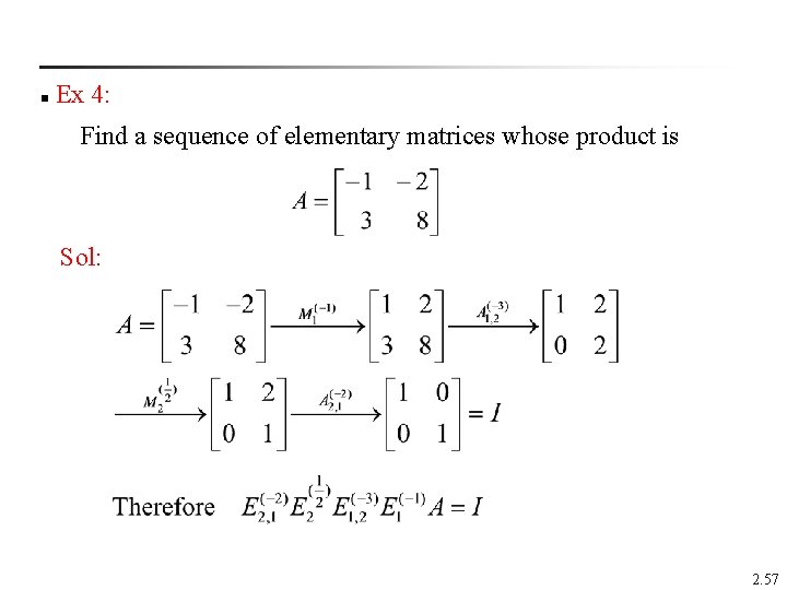
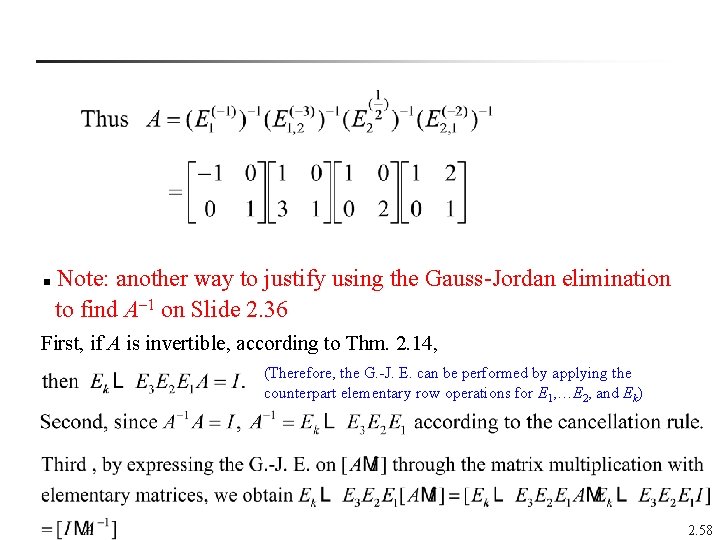
Ex 4: n Find a sequence of elementary matrices whose product is Sol: 2. 57

Note: another way to justify using the Gauss-Jordan elimination to find A– 1 on Slide 2. 36 n First, if A is invertible, according to Thm. 2. 14, (Therefore, the G. -J. E. can be performed by applying the counterpart elementary row operations for E 1, …E 2, and Ek) 2. 58

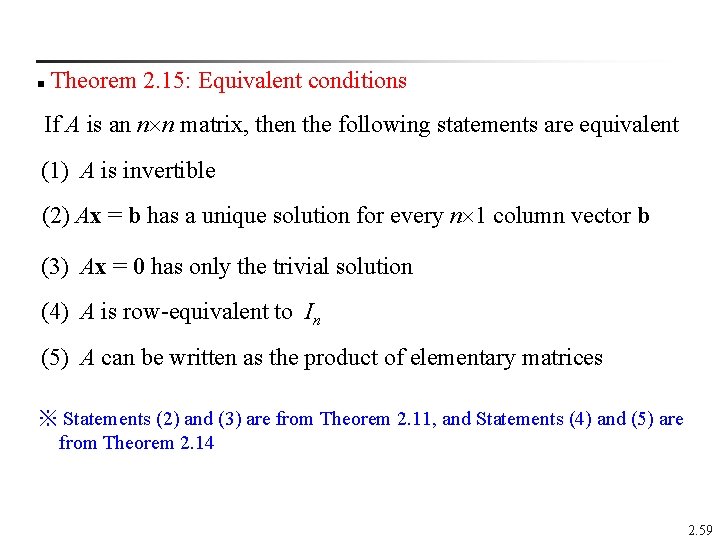
Theorem 2. 15: Equivalent conditions n If A is an n n matrix, then the following statements are equivalent (1) A is invertible (2) Ax = b has a unique solution for every n 1 column vector b (3) Ax = 0 has only the trivial solution (4) A is row-equivalent to In (5) A can be written as the product of elementary matrices ※ Statements (2) and (3) are from Theorem 2. 11, and Statements (4) and (5) are from Theorem 2. 14 2. 59

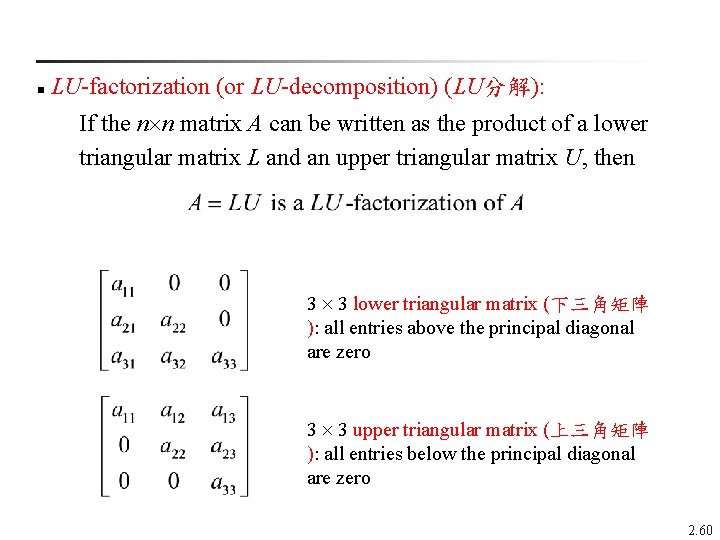
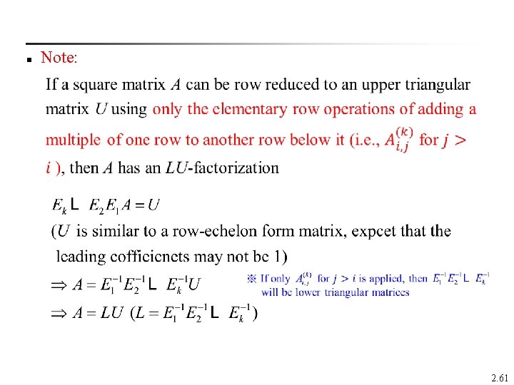
n LU-factorization (or LU-decomposition) (LU分解): If the n n matrix A can be written as the product of a lower triangular matrix L and an upper triangular matrix U, then 3 3 lower triangular matrix (下三角矩陣 ): all entries above the principal diagonal are zero 3 3 upper triangular matrix (上三角矩陣 ): all entries below the principal diagonal are zero 2. 60

n Note: n n 2. 61

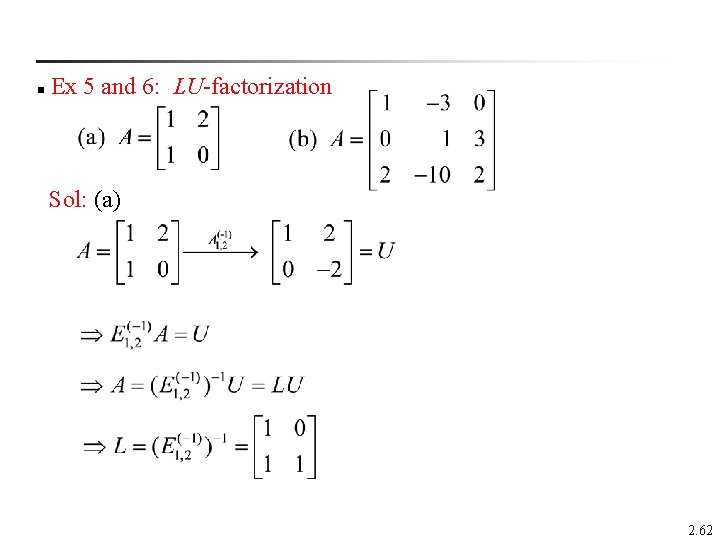
Ex 5 and 6: LU-factorization n Sol: (a) 2. 62

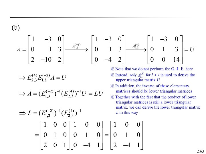
(b) n 2. 63

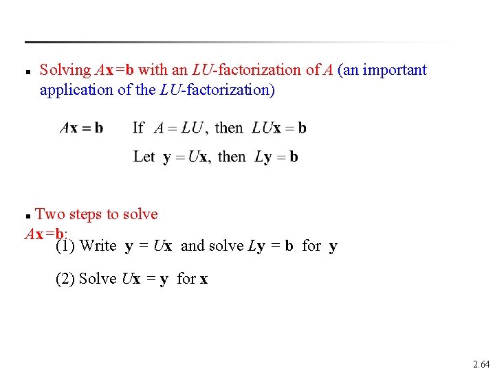
n Solving Ax=b with an LU-factorization of A (an important application of the LU-factorization) Two steps to solve Ax=b: (1) Write y = Ux and solve Ly = b for y n (2) Solve Ux = y for x 2. 64

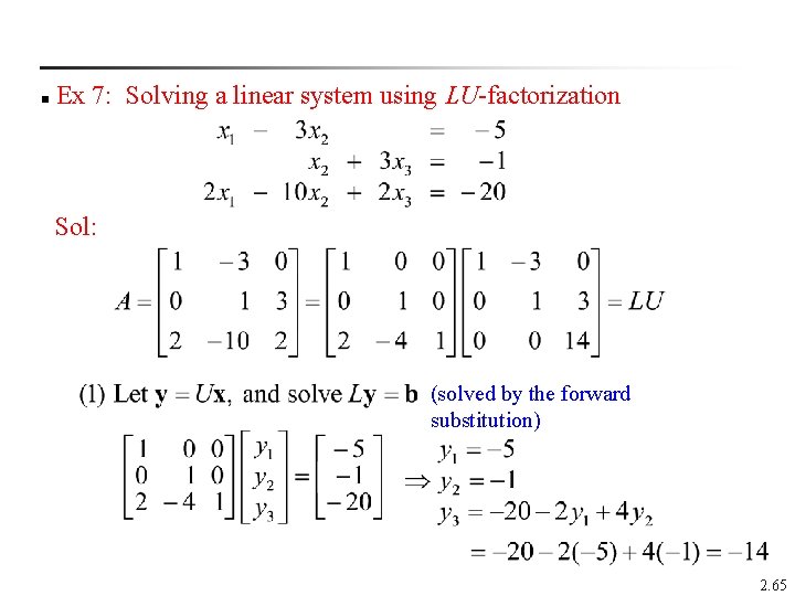
Ex 7: Solving a linear system using LU-factorization n Sol: (solved by the forward substitution) 2. 65

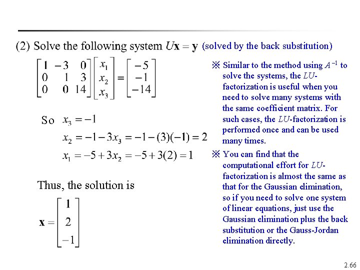
(solved by the back substitution) So Thus, the solution is ※ Similar to the method using A – 1 to solve the systems, the LUfactorization is useful when you need to solve many systems with the same coefficient matrix. For such cases, the LU-factorization is performed once and can be used many times. ※ You can find that the computational effort for LUfactorization is almost the same as that for the Gaussian elimination, so if you need to solve one system of linear equations, just use the Gaussian elimination plus the back substitution or the Gauss-Jordan elimination directly. 2. 66

Keywords in Section 2. 4: n row elementary matrix: 列基本矩陣 n row equivalent: 列等價 n lower triangular matrix: 下三角矩陣 n upper triangular matrix: 上三角矩陣 n LU-factorization: LU分解 2. 67

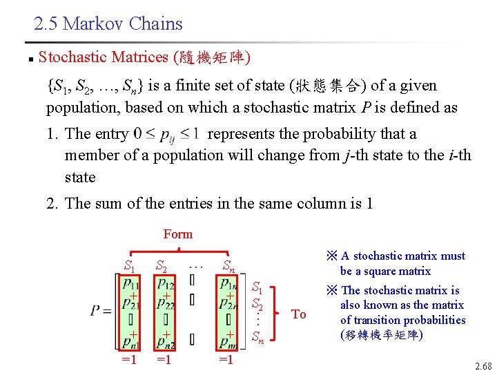
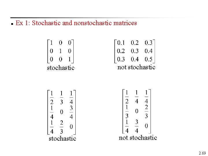
2. 5 Markov Chains n Stochastic Matrices (隨機矩陣) {S 1, S 2, …, Sn} is a finite set of state (狀態集合) of a given population, based on which a stochastic matrix P is defined as 1. The entry represents the probability that a member of a population will change from j-th state to the i-th state 2. The sum of the entries in the same column is 1 Form S 1 S 2 + + … ※ A stochastic matrix must be a square matrix Sn + + + =1 =1 =1 … + S 1 S 2 Sn To ※ The stochastic matrix is also known as the matrix of transition probabilities (移轉機率矩陣) 2. 68

n Ex 1: Stochastic and nonstochastic matrices stochastic not stochastic 2. 69

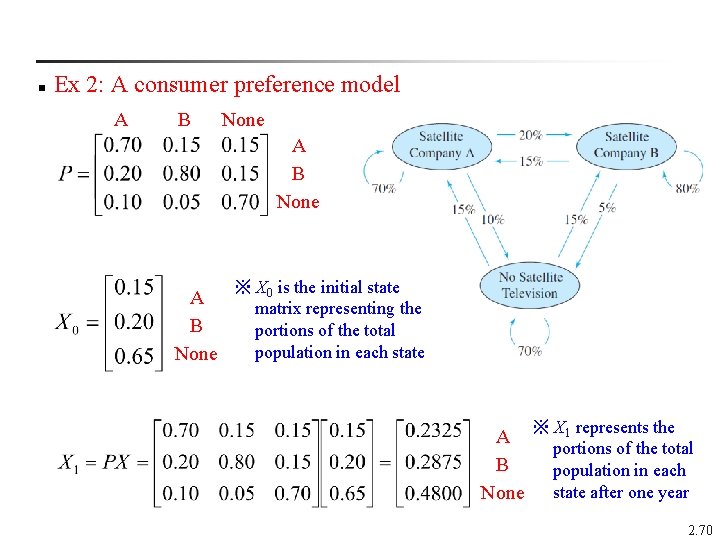
n Ex 2: A consumer preference model A B None A B None ※ X 0 is the initial state matrix representing the portions of the total population in each state A B None ※ X 1 represents the portions of the total population in each state after one year 2. 70

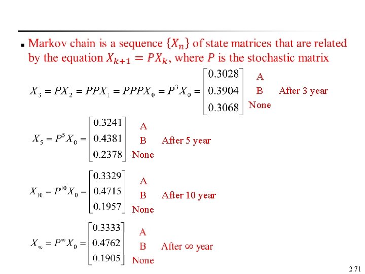
n A B After 3 year None A B After 5 year None A B After 10 year None n 2. 71

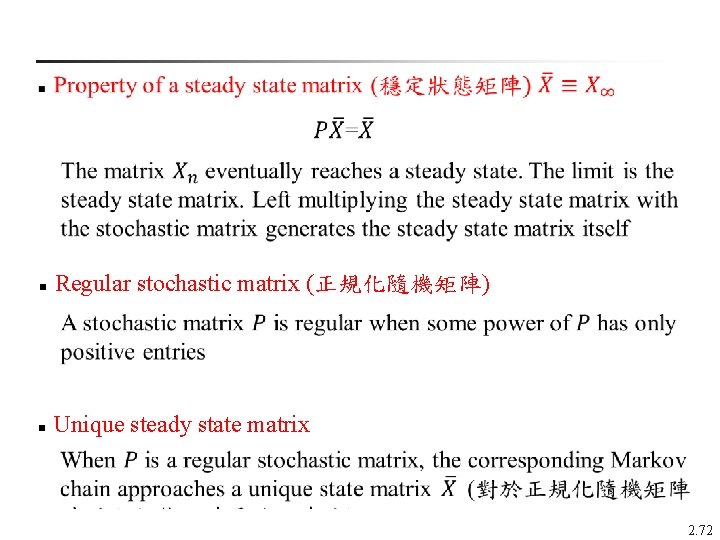
n n n n Regular stochastic matrix (正規化隨機矩陣) n n Unique steady state matrix n 2. 72

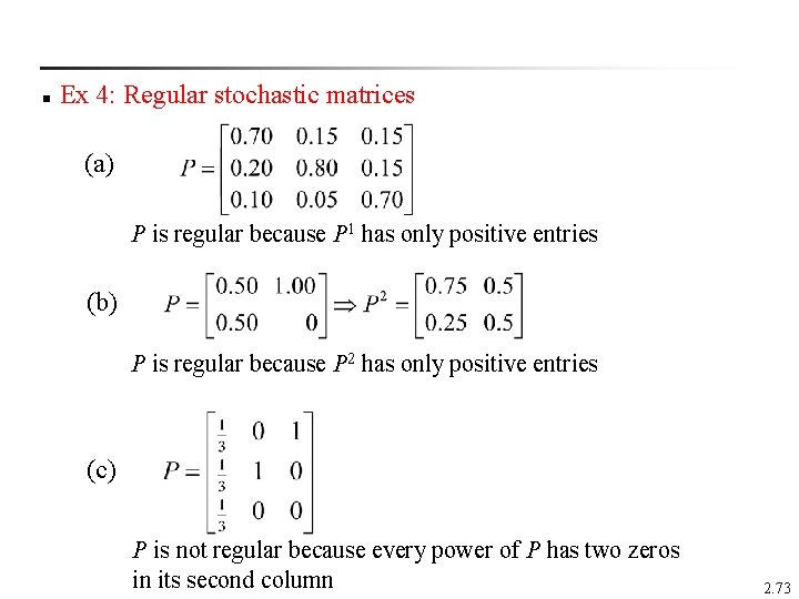
n Ex 4: Regular stochastic matrices (a) P is regular because P 1 has only positive entries (b) P is regular because P 2 has only positive entries (c) P is not regular because every power of P has two zeros in its second column 2. 73

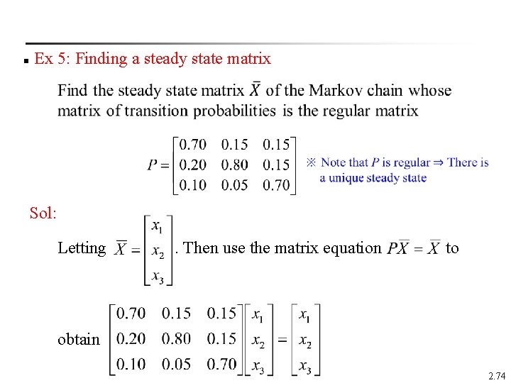
n Ex 5: Finding a steady state matrix n n Sol: Letting . Then use the matrix equation to obtain 2. 74

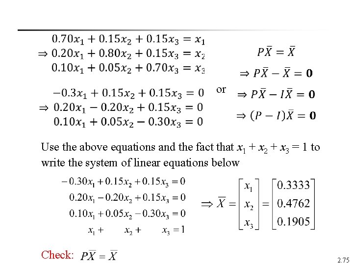
n n n or Use the above equations and the fact that x 1 + x 2 + x 3 = 1 to write the system of linear equations below Check: 2. 75

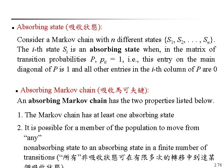
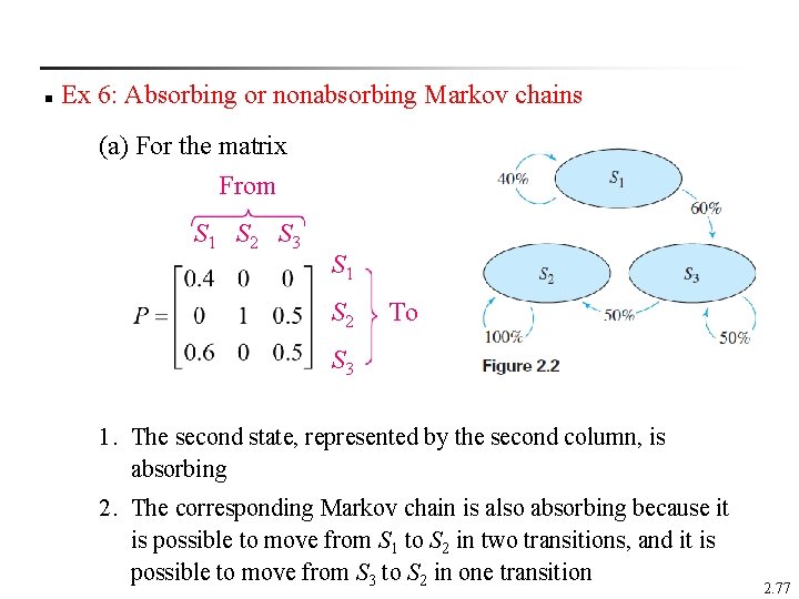
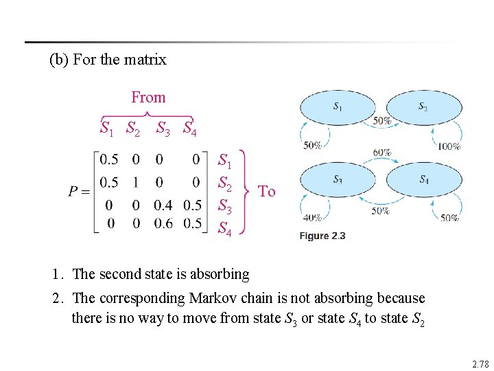
n Absorbing state (吸收狀態): Consider a Markov chain with n different states {S 1, S 2, . . . , Sn}. The i-th state Si is an absorbing state when, in the matrix of transition probabilities P, pii = 1, i. e. , this entry on the main diagonal of P is 1 and all other entries in the i-th column of P are 0 Absorbing Markov chain (吸收馬可夫鏈): An absorbing Markov chain has the two properties listed below. n 1. The Markov chain has at least one absorbing state 2. It is possible for a member of the population to move from “any” nonabsorbing state to an absorbing state in a finite number of transitions (“所有”非吸收狀態可在有限多次的轉移中到達某 2. 76

n Ex 6: Absorbing or nonabsorbing Markov chains (a) For the matrix From S 1 S 2 S 3 S 1 S 2 To S 3 1. The second state, represented by the second column, is absorbing 2. The corresponding Markov chain is also absorbing because it is possible to move from S 1 to S 2 in two transitions, and it is possible to move from S 3 to S 2 in one transition 2. 77

(b) For the matrix From S 1 S 2 S 3 S 4 S 1 S 2 S 3 S 4 To 1. The second state is absorbing 2. The corresponding Markov chain is not absorbing because there is no way to move from state S 3 or state S 4 to state S 2 2. 78

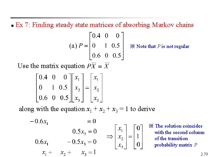
n Ex 7: Finding steady state matrices of absorbing Markov chains ※ Note that P is not regular Use the matrix equation along with the equation x 1 + x 2 + x 3 = 1 to derive ※ The solution coincides with the second column of the transition probability matrix P 2. 79

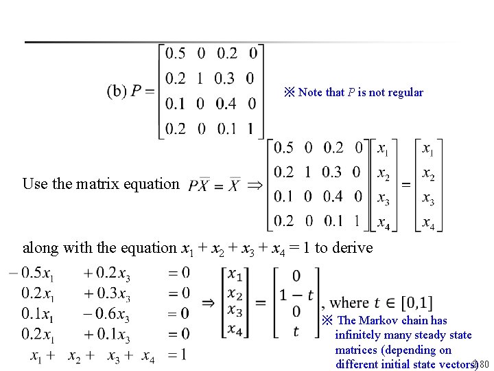
※ Note that P is not regular Use the matrix equation along with the equation x 1 + x 2 + x 3 + x 4 = 1 to derive n ※ The Markov chain has infinitely many steady state matrices (depending on 2. 80 different initial state vectors)

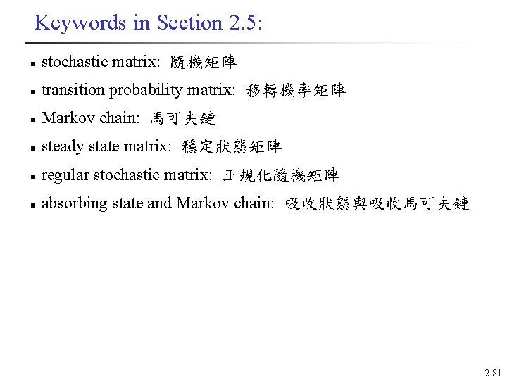
Keywords in Section 2. 5: n stochastic matrix: 隨機矩陣 n transition probability matrix: 移轉機率矩陣 n Markov chain: 馬可夫鏈 n steady state matrix: 穩定狀態矩陣 n regular stochastic matrix: 正規化隨機矩陣 n absorbing state and Markov chain: 吸收狀態與吸收馬可夫鏈 2. 81

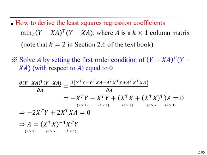
2. 6 Applications of Matrix Operations n Least Squares Regression Analysis (Example 10 in the text book vs. the linear regression in EXCEL) l l Read the text book or “Applications in Ch 2. pdf” downloaded from my website See “Example 10 for regression in Ch 2. xlsx” downloaded from my website for example 2. 82

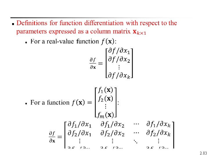
n 2. 83

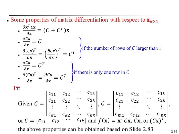
n n n Pf: 2. 84

n n n n n 2. 85

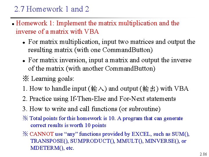
2. 7 Homework 1 and 2 n Homework 1: Implement the matrix multiplication and the inverse of a matrix with VBA u For matrix multiplication, input two matrices and output the resulting matrix (with one Command. Button) u For matrix inversion, input a matrix and output the inverse of the matrix (with another Command. Button) ※ Learning goals: 1. How to handle input (輸入) and output (輸出) with VBA 2. Practice using If-Then-Else and For-Next statements 3. How to write and call functions (or subroutine) ※ Total points for this homework is 10. A program that can generate correct results is worth 10 points ※ CANNOT use “any” functions provided by EXCEL, such as SUM(), TRANSPOSE(), SUMPRODUCT(), MMULT(), MINVERSE(), or MDETERM(), etc. 2. 86

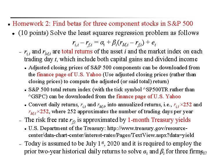
n Homework 2: Find betas for three component stocks in S&P 500 u (10 points) Solve the least squares regression problem as follows ri, t – rf, t = αi + βi(r. M, t – rf, t) + et – ri, t and r. M, t are total returns of the asset i and the market index on each trading day t, which include both capital gains and dividend income l l l – The risk free rate rf, t is approximated by 1 -month Treasury yields l – Adjusted closing prices of S&P 500 components can be downloaded from the finance page of U. S. Yahoo (Use adjusted closing prices (rather than closing prices) to compute the adjusted (or said total) return) S&P 500 total return index (with the tick symbol ^SP 500 TR rather than ^GSPC) can be downloaded from the finance page of U. S. Yahoo Convert daily returns, ri, t and r. M, t, into annualized returns, i. e. , ri, t × 252 and r. M, t × 252, where 252 approximates the number of trading days per year U. S. Department of the Treasury: http: //www. treasury. gov/resourcecenter/data-chart-center/interest-rates/Pages/Text. View. aspx? data=yield Today is assumed to be July 1 st, 2020 and it is required to employ the prior two-year historical daily returns to solve αi and βi for three firms 2. 87

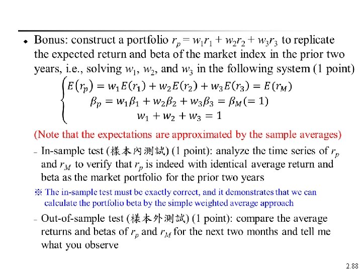
n 2. 88

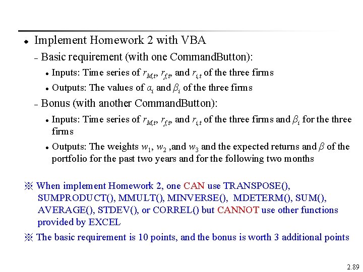
u Implement Homework 2 with VBA – Basic requirement (with one Command. Button): l l – Inputs: Time series of r. M, t, rf, t, and ri, t of the three firms Outputs: The values of αi and βi of the three firms Bonus (with another Command. Button): l l Inputs: Time series of r. M, t, rf, t, and ri, t of the three firms and βi for the three firms Outputs: The weights w 1, w 2 , and w 3 and the expected returns and β of the portfolio for the past two years and for the following two months ※ When implement Homework 2, one CAN use TRANSPOSE(), SUMPRODUCT(), MMULT(), MINVERSE(), MDETERM(), SUM(), AVERAGE(), STDEV(), or CORREL() but CANNOT use other functions provided by EXCEL ※ The basic requirement is 10 points, and the bonus is worth 3 additional points 2. 89