ME 521 Computer Aided Design 5 Curves and

ME 521 Computer Aided Design 5. Curves and Curve Modeling Assoc. Dr. Ahmet Zafer Şenalp e-mail: azsenalp@gmail. com Mechanical Engineering Department Gebze Technical University

5. Curves and Curve Modeling Purpose Ø Curves are the basics for surfaces Ø Before learning surfaces curves have to be known Ø When asked to modify a particular entity on a CAD system, knowledge of the entities can increase your productivity Ø Understand how the math presentation of various curve entities relates to a user interface Ø Understand what is impossible and which way can be more efficient when creating or modifying an entity Dr. Ahmet Zafer Şenalp ME 521 Mechanical Engineering Department, GTU 2

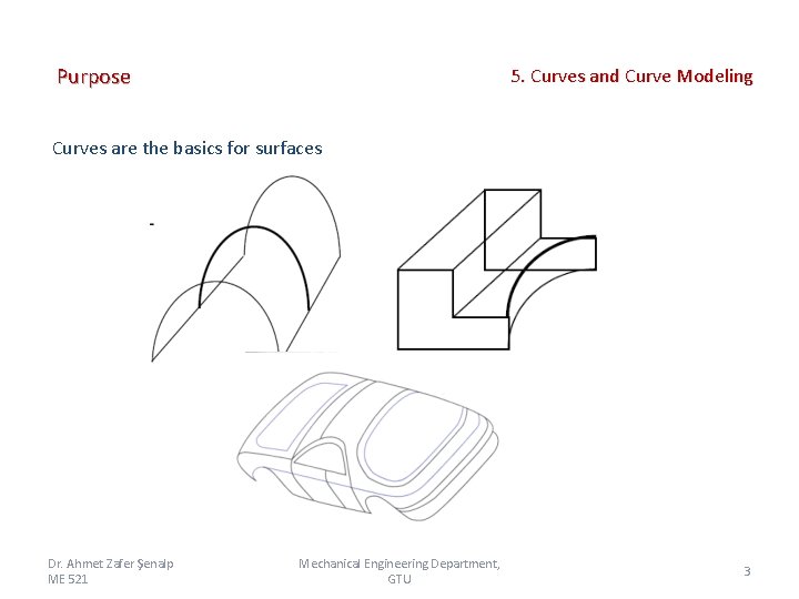
5. Curves and Curve Modeling Purpose Curves are the basics for surfaces Dr. Ahmet Zafer Şenalp ME 521 Mechanical Engineering Department, GTU 3

Why Not Simply Use a Point Matrix to Represent a Curve? 5. Curves and Curve Modeling Ø Storage issue and limited resolution Ø Computation and transformation Ø Difficulties in calculating the intersections or curves and physical properties of objects Ø Difficulties in design (e. g. control shapes of an existing object) Ø Poor surface finish of manufactured parts Dr. Ahmet Zafer Şenalp ME 521 Mechanical Engineering Department, GTU 4

Advantages of Analytical Representation for Geometric Entities 5. Curves and Curve Modeling Ø A few parameters to store Ø Designers know the effect of data points on curve behavior, control, continuity, and curvature Ø Facilitate calculations of intersections, object properties, etc. Dr. Ahmet Zafer Şenalp ME 521 Mechanical Engineering Department, GTU 5

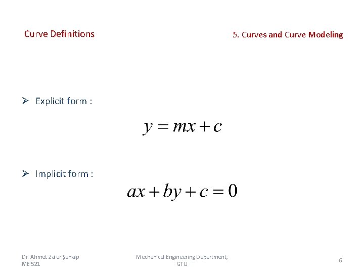
Curve Definitions 5. Curves and Curve Modeling Ø Explicit form : Ø Implicit form : Dr. Ahmet Zafer Şenalp ME 521 Mechanical Engineering Department, GTU 6

Drawbacks of Conventional Representations 5. Curves and Curve Modeling Conventional explicit and implicit forms have several drawbacks. Ø Ø They represent unbounded geometry They may be multi-valued Difficult to evaluate points along the curve Depends on coordinate system Dr. Ahmet Zafer Şenalp ME 521 Mechanical Engineering Department, GTU 7

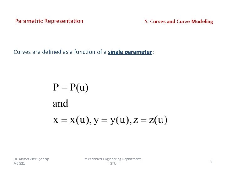
Parametric Representation 5. Curves and Curve Modeling Curves are defined as a function of a single parameter: Dr. Ahmet Zafer Şenalp ME 521 Mechanical Engineering Department, GTU 8

Parametric Representation 5. Curves and Curve Modeling u Curve, P=P(u)=[x(u), y(u), z(u)]T u Surface, P=P(u, v) v P(u, v)=[x(u, v), y(u, v), z(u, v)]T Dr. Ahmet Zafer Şenalp ME 521 Mechanical Engineering Department, GTU 9

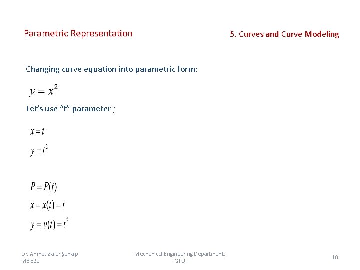
Parametric Representation 5. Curves and Curve Modeling Changing curve equation into parametric form: Let’s use “t” parameter ; Dr. Ahmet Zafer Şenalp ME 521 Mechanical Engineering Department, GTU 10

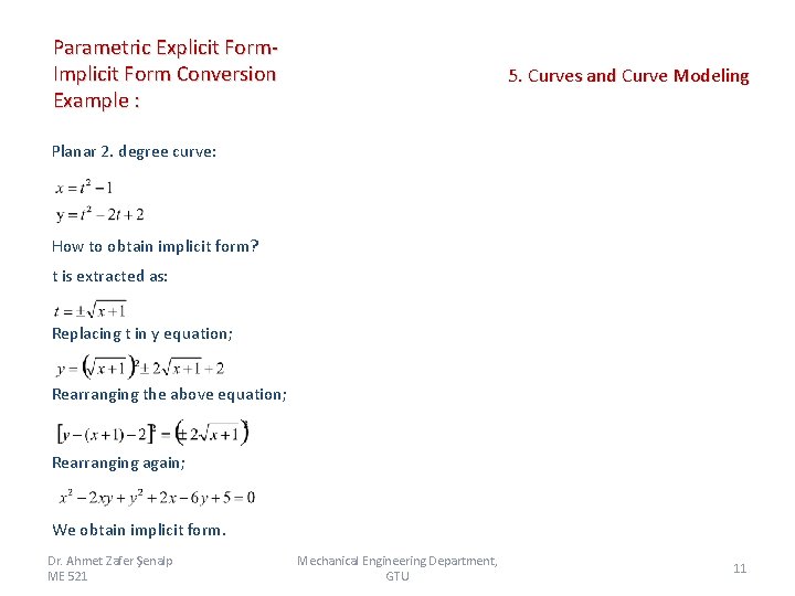
Parametric Explicit Form. Implicit Form Conversion Example : 5. Curves and Curve Modeling Planar 2. degree curve: How to obtain implicit form? t is extracted as: Replacing t in y equation; Rearranging the above equation; Rearranging again; We obtain implicit form. Dr. Ahmet Zafer Şenalp ME 521 Mechanical Engineering Department, GTU 11

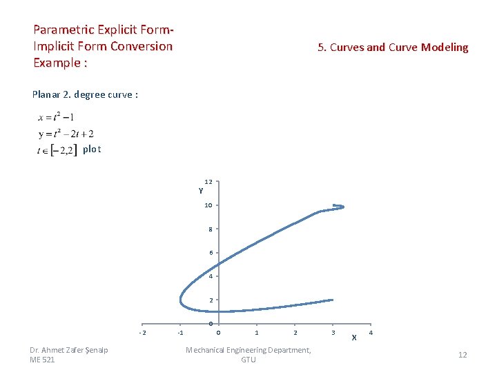
Parametric Explicit Form. Implicit Form Conversion Example : 5. Curves and Curve Modeling Planar 2. degree curve : plot 12 Y 10 8 6 4 2 0 -2 Dr. Ahmet Zafer Şenalp ME 521 -1 0 1 2 Mechanical Engineering Department, GTU 3 X 4 12

Curve Classification 5. Curves and Curve Modeling Curve Classification: Ø Analytic Curves Ø Synthetic curves Dr. Ahmet Zafer Şenalp ME 521 Mechanical Engineering Department, GTU 13

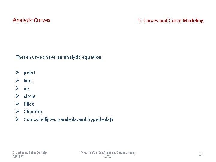
Analytic Curves 5. Curves and Curve Modeling These curves have an analytic equation Ø Ø Ø Ø point line arc circle fillet Chamfer Conics (ellipse, parabola, and hyperbola)) Dr. Ahmet Zafer Şenalp ME 521 Mechanical Engineering Department, GTU 14

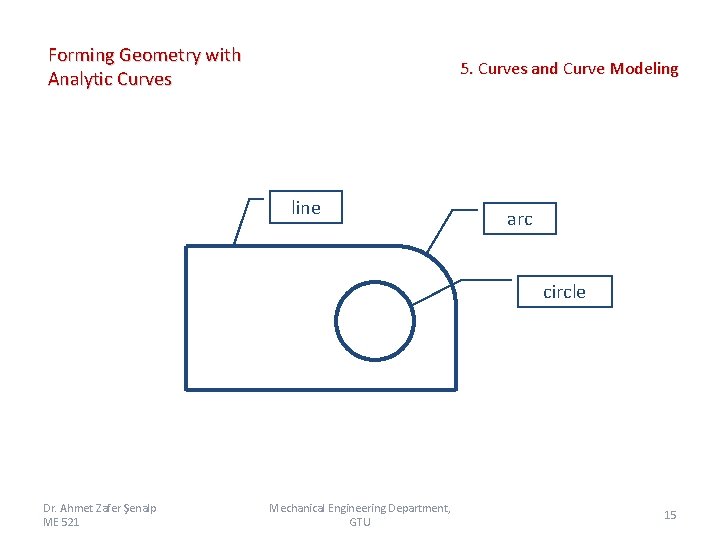
Forming Geometry with Analytic Curves 5. Curves and Curve Modeling line arc circle Dr. Ahmet Zafer Şenalp ME 521 Mechanical Engineering Department, GTU 15

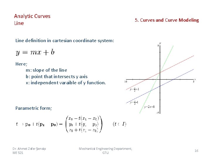
Analytic Curves Line 5. Curves and Curve Modeling Line definition in cartesian coordinate system: Here; m: slope of the line b: point that intersects y axis x: independent varaible of y function. Parametric form; Dr. Ahmet Zafer Şenalp ME 521 Mechanical Engineering Department, GTU 16

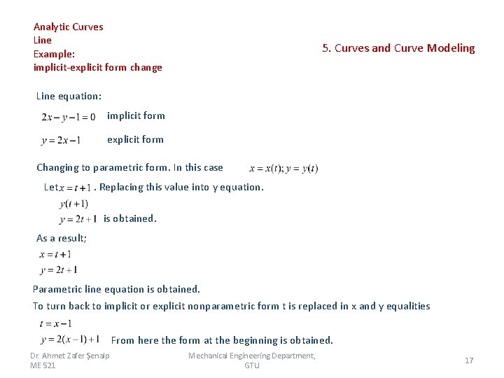
Analytic Curves Line Example: implicit-explicit form change 5. Curves and Curve Modeling Line equation: implicit form explicit form Changing to parametric form. In this case Let . Replacing this value into y equation. is obtained. As a result; Parametric line equation is obtained. To turn back to implicit or explicit nonparametric form t is replaced in x and y equalities From here the form at the beginning is obtained. Dr. Ahmet Zafer Şenalp ME 521 Mechanical Engineering Department, GTU 17

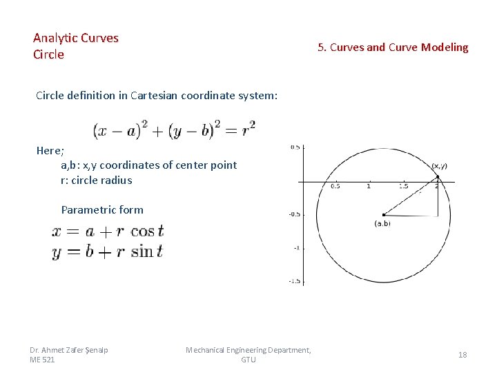
Analytic Curves Circle 5. Curves and Curve Modeling Circle definition in Cartesian coordinate system: Here; a, b: x, y coordinates of center point r: circle radius Parametric form Dr. Ahmet Zafer Şenalp ME 521 Mechanical Engineering Department, GTU 18

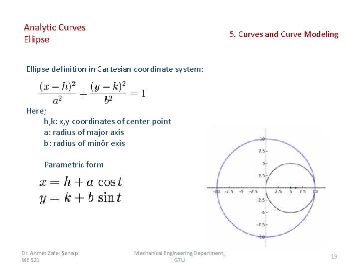
Analytic Curves Ellipse 5. Curves and Curve Modeling Ellipse definition in Cartesian coordinate system: Here; h, k: x, y coordinates of center point a: radius of major axis b: radius of minör exis Parametric form Dr. Ahmet Zafer Şenalp ME 521 Mechanical Engineering Department, GTU 19

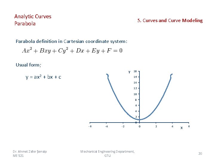
Analytic Curves Parabola 5. Curves and Curve Modeling Parabola definition in Cartesian coordinate system: Usual form; Y 18 y = ax 2 + bx + c 16 14 12 10 8 6 4 2 0 -6 Dr. Ahmet Zafer Şenalp ME 521 -4 -2 Mechanical Engineering Department, GTU 0 2 4 X 6 20

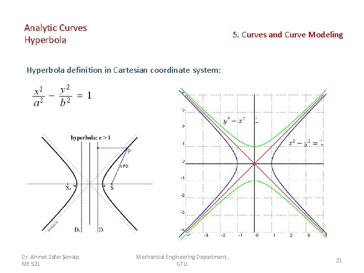
Analytic Curves Hyperbola 5. Curves and Curve Modeling Hyperbola definition in Cartesian coordinate system: Dr. Ahmet Zafer Şenalp ME 521 Mechanical Engineering Department, GTU 21

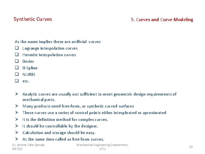
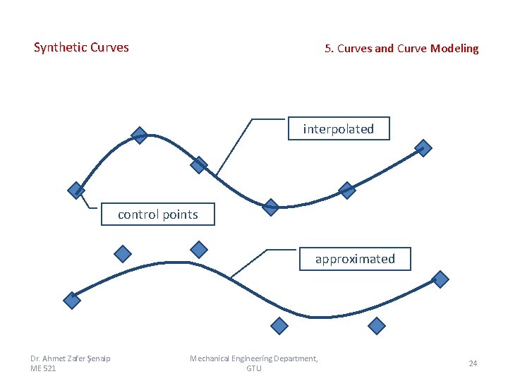
Synthetic Curves 5. Curves and Curve Modeling As the name implies these artificial curves q Lagrange interpolation curves q Hermite interpolation curves q Bezier q B-Spline q NURBS q etc. Ø Analytic curves are usually not sufficient to meet geometric design requirements of mechanical parts. Ø Many products need free-form, or synthetic curved surfaces Ø These curves use a series of control points either interploated or aproximated Ø It is the definition method for complex curves. Ø It should be controllable by the designer. Ø Calculation and storage should be easy. Ø At the same time called as free form curves. Dr. Ahmet Zafer Şenalp ME 521 Mechanical Engineering Department, GTU 22

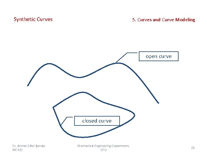
Synthetic Curves 5. Curves and Curve Modeling open curve closed curve Dr. Ahmet Zafer Şenalp ME 521 Mechanical Engineering Department, GTU 23

Synthetic Curves 5. Curves and Curve Modeling interpolated control points approximated Dr. Ahmet Zafer Şenalp ME 521 Mechanical Engineering Department, GTU 24

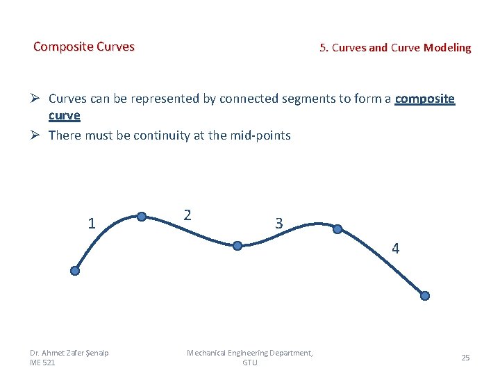
Composite Curves 5. Curves and Curve Modeling Ø Curves can be represented by connected segments to form a composite curve Ø There must be continuity at the mid-points 1 2 3 4 Dr. Ahmet Zafer Şenalp ME 521 Mechanical Engineering Department, GTU 25

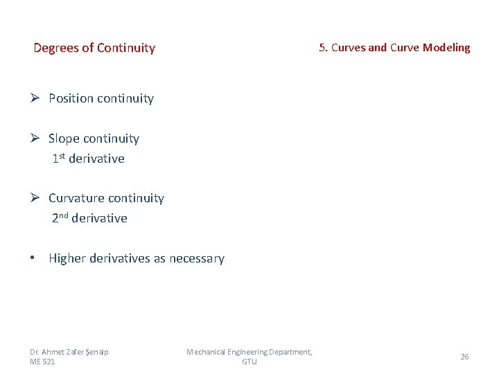
Degrees of Continuity 5. Curves and Curve Modeling Ø Position continuity Ø Slope continuity 1 st derivative Ø Curvature continuity 2 nd derivative • Higher derivatives as necessary Dr. Ahmet Zafer Şenalp ME 521 Mechanical Engineering Department, GTU 26

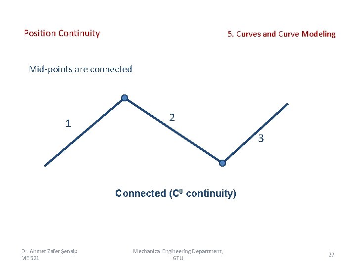
Position Continuity 5. Curves and Curve Modeling Mid-points are connected 1 2 3 Connected (C 0 continuity) Dr. Ahmet Zafer Şenalp ME 521 Mechanical Engineering Department, GTU 27

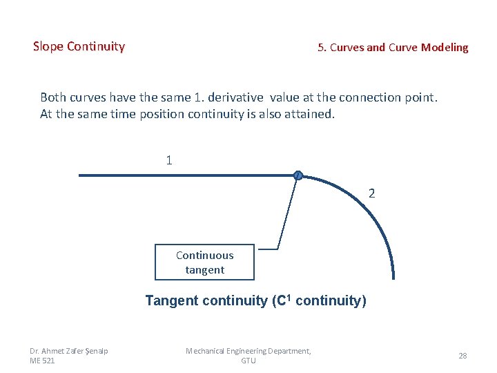
Slope Continuity 5. Curves and Curve Modeling Both curves have the same 1. derivative value at the connection point. At the same time position continuity is also attained. 1 2 Continuous tangent Tangent continuity (C 1 continuity) Dr. Ahmet Zafer Şenalp ME 521 Mechanical Engineering Department, GTU 28

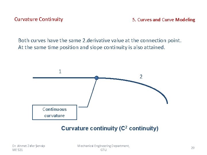
Curvature Continuity 5. Curves and Curve Modeling Both curves have the same 2. derivative value at the connection point. At the same time position and slope continuity is also attained. 1 2 Continuous curvature Curvature continuity (C 2 continuity) Dr. Ahmet Zafer Şenalp ME 521 Mechanical Engineering Department, GTU 29

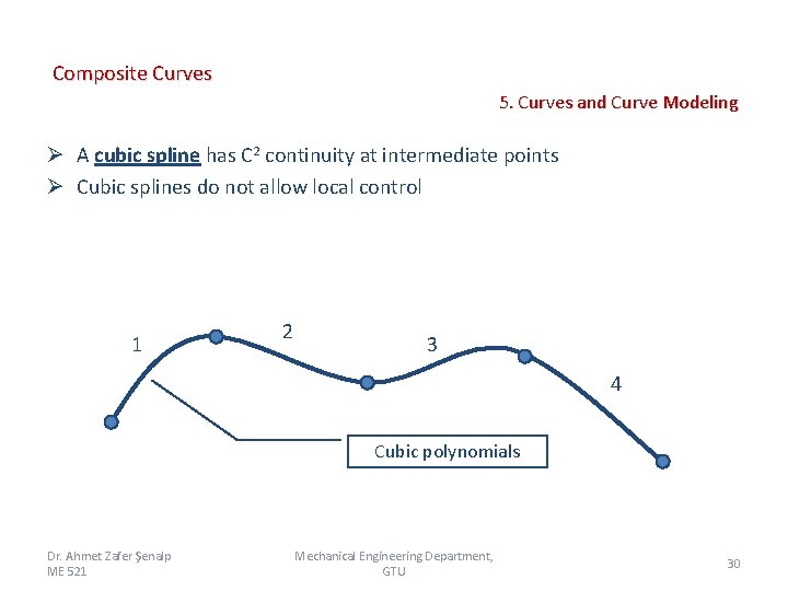
Composite Curves 5. Curves and Curve Modeling Ø A cubic spline has C 2 continuity at intermediate points Ø Cubic splines do not allow local control 1 2 3 4 Cubic polynomials Dr. Ahmet Zafer Şenalp ME 521 Mechanical Engineering Department, GTU 30

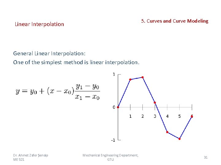
5. Curves and Curve Modeling Linear Interpolation General Linear Interpolation: One of the simplest method is linear interpolation. Dr. Ahmet Zafer Şenalp ME 521 Mechanical Engineering Department, GTU 31

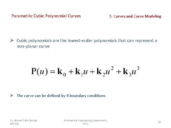
Parametric Cubic Polynomial Curves 5. Curves and Curve Modeling Ø Cubic polynomials are the lowest-order polynomials that can represent a non-planar curve Ø The curve can be defined by 4 boundary conditions Dr. Ahmet Zafer Şenalp ME 521 Mechanical Engineering Department, GTU 32

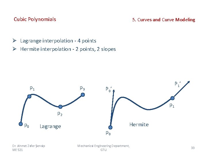
Cubic Polynomials 5. Curves and Curve Modeling Ø Lagrange interpolation - 4 points Ø Hermite interpolation - 2 points, 2 slopes p 1 p 3 P 1 ’ P 0 ’ p 1 p 2 p 0 Lagrange Dr. Ahmet Zafer Şenalp ME 521 Hermite p 0 Mechanical Engineering Department, GTU 33

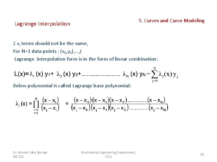
5. Curves and Curve Modeling Lagrange Interpolation 2 xi terms should not be the same, For N+1 data points ; (x 0, y 0), . . . , (x. N, y. N) için Lagrange interpolation form is in the form of linear combination: Below polynomial is called Lagrange base polynomial; Dr. Ahmet Zafer Şenalp ME 521 Mechanical Engineering Department, GTU 34

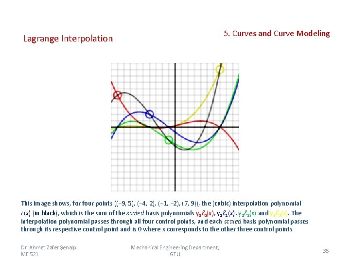
5. Curves and Curve Modeling Lagrange Interpolation This image shows, for four points ((− 9, 5), (− 4, 2), (− 1, − 2), (7, 9)), the (cubic) interpolation polynomial L(x) (in black), which is the sum of the scaled basis polynomials y 0ℓ 0(x), y 1ℓ 1(x), y 2ℓ 2(x) and y 3ℓ 3(x). The interpolation polynomial passes through all four control points, and each scaled basis polynomial passes through its respective control point and is 0 where x corresponds to the other three control points Dr. Ahmet Zafer Şenalp ME 521 Mechanical Engineering Department, GTU 35

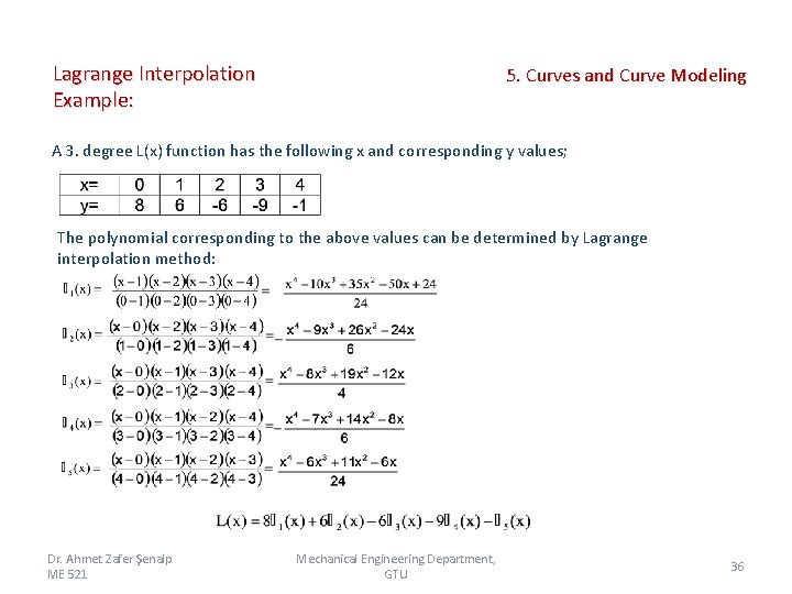
Lagrange Interpolation Example: 5. Curves and Curve Modeling A 3. degree L(x) function has the following x and corresponding y values; The polynomial corresponding to the above values can be determined by Lagrange interpolation method: Dr. Ahmet Zafer Şenalp ME 521 Mechanical Engineering Department, GTU 36

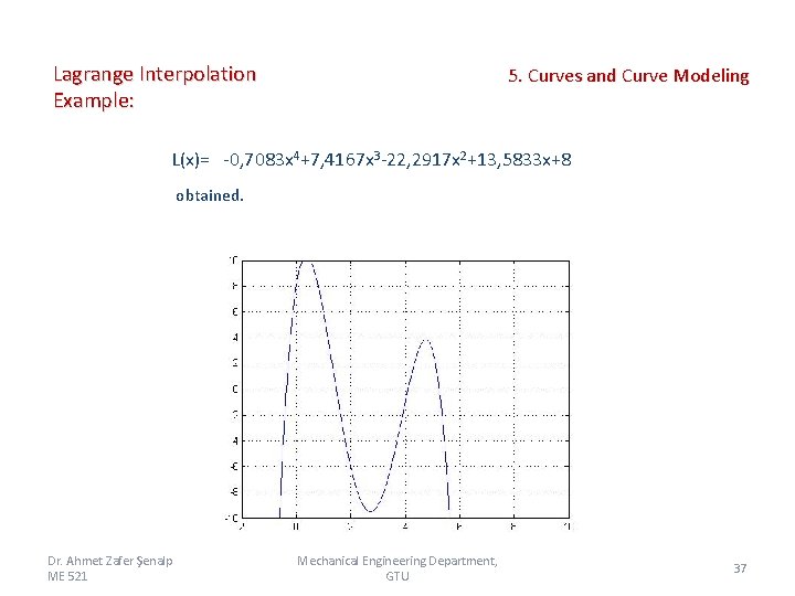
Lagrange Interpolation Example: 5. Curves and Curve Modeling L(x)= -0, 7083 x 4+7, 4167 x 3 -22, 2917 x 2+13, 5833 x+8 obtained. Dr. Ahmet Zafer Şenalp ME 521 Mechanical Engineering Department, GTU 37

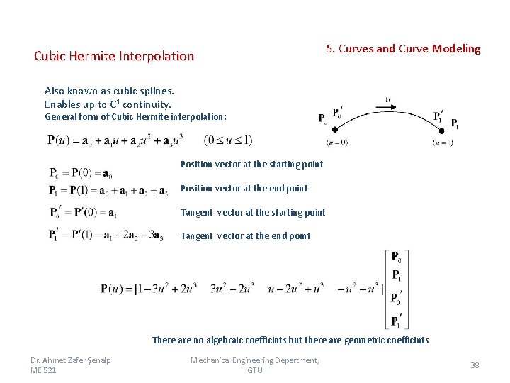
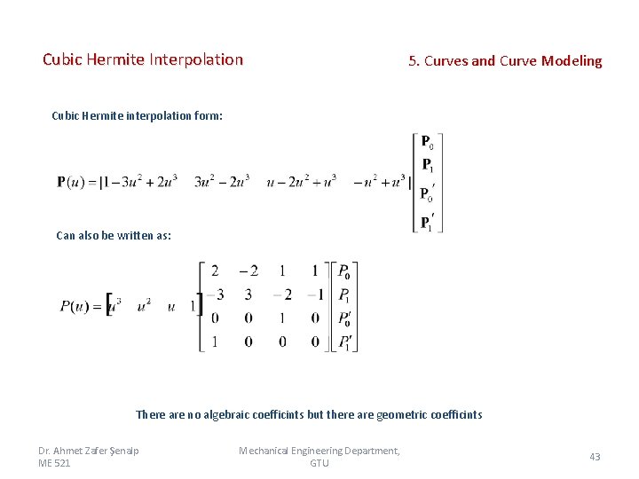
Cubic Hermite Interpolation 5. Curves and Curve Modeling Also known as cubic splines. Enables up to C 1 continuity. General form of Cubic Hermite interpolation: Position vector at the starting point Position vector at the end point Tangent vector at the starting point Tangent vector at the end point There are no algebraic coefficints but there are geometric coefficints Dr. Ahmet Zafer Şenalp ME 521 Mechanical Engineering Department, GTU 38

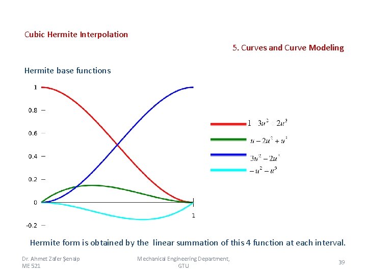
Cubic Hermite Interpolation 5. Curves and Curve Modeling Hermite base functions Hermite form is obtained by the linear summation of this 4 function at each interval. Dr. Ahmet Zafer Şenalp ME 521 Mechanical Engineering Department, GTU 39

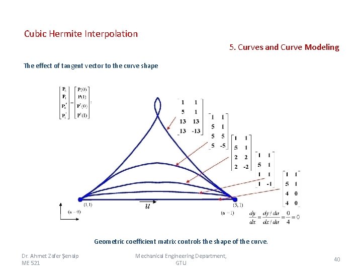
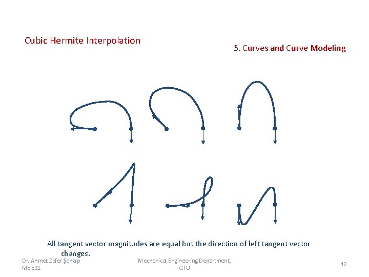
Cubic Hermite Interpolation 5. Curves and Curve Modeling The effect of tangent vector to the curve shape Geometrik katsayı matrisi Geometric coefficient matrix controls the shape of the curve. Dr. Ahmet Zafer Şenalp ME 521 Mechanical Engineering Department, GTU 40

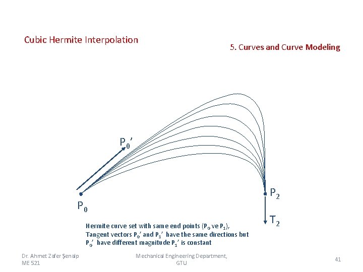
Cubic Hermite Interpolation 5. Curves and Curve Modeling P 0’ P 2 P 0 Hermite curve set with same end points (P 0 ve P 1), Tangent vectors P 0’ and P 1’ have the same directions but P 0’ have different magnitude P 1’ is constant Dr. Ahmet Zafer Şenalp ME 521 Mechanical Engineering Department, GTU T 2 41

Cubic Hermite Interpolation 5. Curves and Curve Modeling All tangent vector magnitudes are equal but the direction of left tangent vector changes. Dr. Ahmet Zafer Şenalp ME 521 Mechanical Engineering Department, GTU 42

Cubic Hermite Interpolation 5. Curves and Curve Modeling Cubic Hermite interpolation form: Can also be written as: There are no algebraic coefficints but there are geometric coefficints Dr. Ahmet Zafer Şenalp ME 521 Mechanical Engineering Department, GTU 43

Approximated Curves q q 5. Curves and Curve Modeling Bezier B-Spline NURBS etc. Dr. Ahmet Zafer Şenalp ME 521 Mechanical Engineering Department, GTU 44

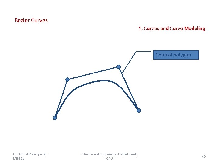
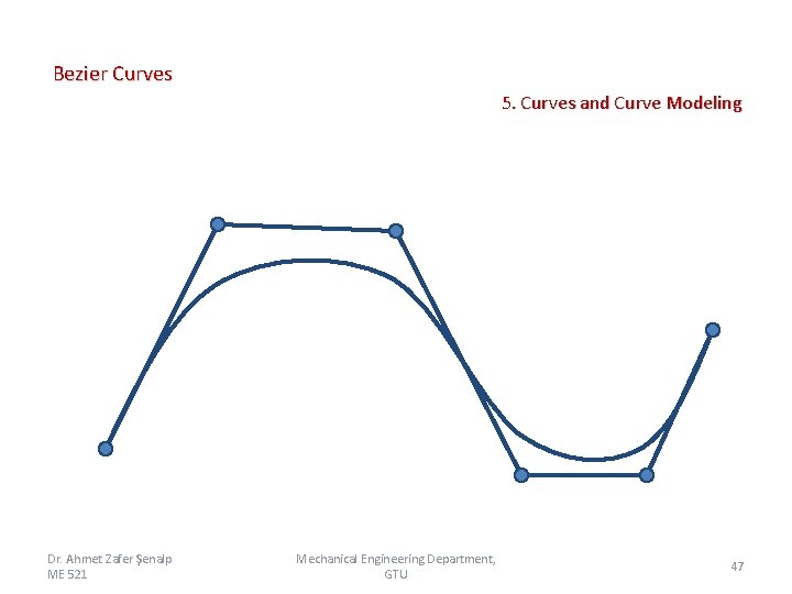
Bezier Curves 5. Curves and Curve Modeling Ø P. Bezier of the French automobile company of Renault first introduced the Bezier curve (1962). Ø Bezier curves were developed to allow more convenient manipulation of curves Ø A system for designing sculptured surfaces of automobile bodies (based on the Bezier curve) Ø A Bezier curve is a polynomial curve approximating a control polygon Ø Quadratic and cubic Bézier curves are most common Ø Higher degree curves are more expensive to evaluate. Ø When more complex shapes are needed, low order Bézier curves are patched together. Ø Bézier curves are easily programmable. Bezier curves are widely used in computer graphics. Ø Enables up to C 1 continuity. Dr. Ahmet Zafer Şenalp ME 521 Mechanical Engineering Department, GTU 45

Bezier Curves 5. Curves and Curve Modeling Control polygon Dr. Ahmet Zafer Şenalp ME 521 Mechanical Engineering Department, GTU 46

Bezier Curves 5. Curves and Curve Modeling Dr. Ahmet Zafer Şenalp ME 521 Mechanical Engineering Department, GTU 47

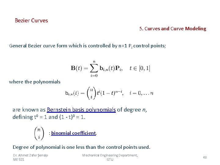
Bezier Curves 5. Curves and Curve Modeling General Bezier curve form which is controlled by n+1 Pi control points; where the polynomials are known as Bernstein basis polynomials of degree n, defining t 0 = 1 and (1 - t)0 = 1. : binomial coefficient. Degree of polynomial is one less than the control points used. Dr. Ahmet Zafer Şenalp ME 521 Mechanical Engineering Department, GTU 48

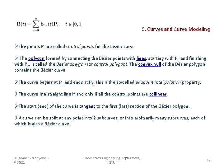
5. Curves and Curve Modeling ØThe points Pi are called control points for the Bézier curve Ø The polygon formed by connecting the Bézier points with lines, starting with P 0 and finishing with Pn, is called the Bézier polygon (or control polygon). The convex hull of the Bézier polygon contains the Bézier curve. ØThe curve begins at P 0 and ends at Pn; this is the so-called endpoint interpolation property. ØThe curve is a straight line if and only if all the control points are collinear. ØThe start (end) of the curve is tangent to the first (last) section of the Bézier polygon. ØA curve can be split at any point into 2 subcurves, or into arbitrarily many subcurves, each of which is also a Bézier curve. Dr. Ahmet Zafer Şenalp ME 521 Mechanical Engineering Department, GTU 49

Bezier Curves Linear Curves 5. Curves and Curve Modeling t= [0, 1] form of a linear Bézier curve turns out to be linear interpollation form. Curve passes through points P 0 ve P 1. Animation of a linear Bézier curve, t in [0, 1]. The t in the function for a linear Bézier curve can be thought of as describing how far B(t) is from P 0 to P 1. For example when t=0. 25, B(t) is one quarter of the way from point P 0 to P 1. As t varies from 0 to 1, B(t) describes a curved line from P 0 to P 1. Dr. Ahmet Zafer Şenalp ME 521 Mechanical Engineering Department, GTU 50

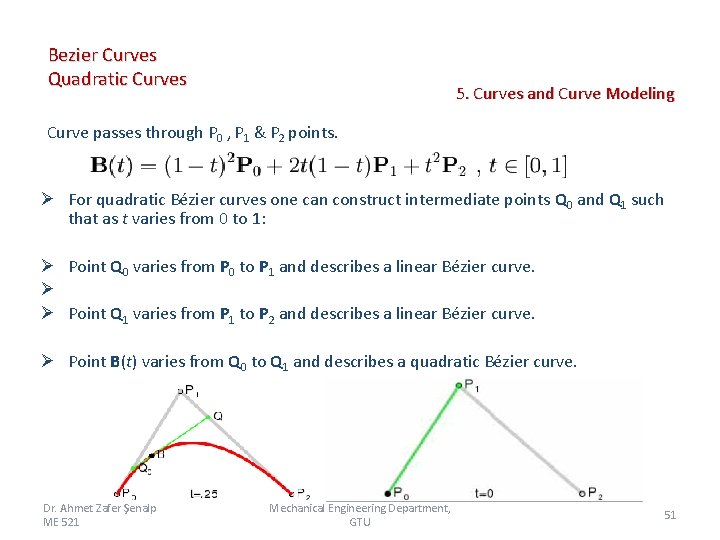
Bezier Curves Quadratic Curves 5. Curves and Curve Modeling Curve passes through P 0 , P 1 & P 2 points. Ø For quadratic Bézier curves one can construct intermediate points Q 0 and Q 1 such that as t varies from 0 to 1: Ø Point Q 0 varies from P 0 to P 1 and describes a linear Bézier curve. Ø Ø Point Q 1 varies from P 1 to P 2 and describes a linear Bézier curve. Ø Point B(t) varies from Q 0 to Q 1 and describes a quadratic Bézier curve. Dr. Ahmet Zafer Şenalp ME 521 Mechanical Engineering Department, GTU 51

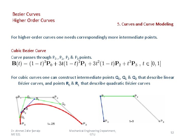
Bezier Curves Higher Order Curves 5. Curves and Curve Modeling For higher-order curves one needs correspondingly more intermediate points. Cubic Bezier Curve passes through P 0 , P 1, P 2 & P 3 points. For cubic curves one can construct intermediate points Q 0, Q 1 & Q 2 that describe linear Bézier curves, and points R 0 & R 1 that describe quadratic Bézier curves Dr. Ahmet Zafer Şenalp ME 521 Mechanical Engineering Department, GTU 52

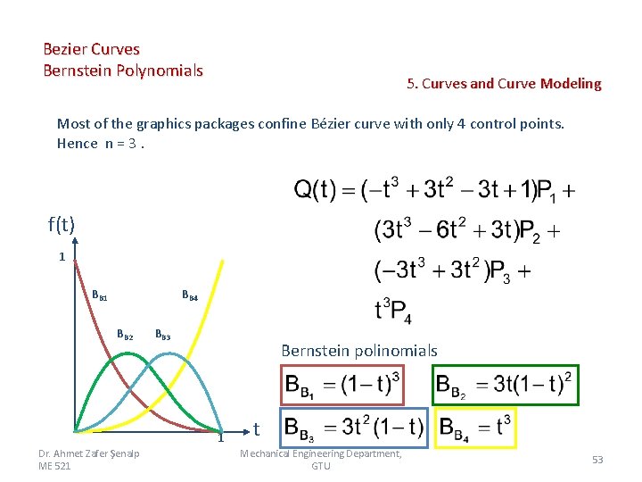
Bezier Curves Bernstein Polynomials 5. Curves and Curve Modeling Most of the graphics packages confine Bézier curve with only 4 control points. Hence n = 3. f(t) 1 BB 4 BB 2 BB 3 Bernstein polinomials 1 Dr. Ahmet Zafer Şenalp ME 521 t Mechanical Engineering Department, GTU 53

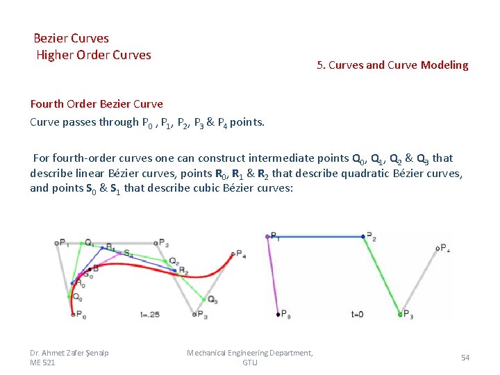
Bezier Curves Higher Order Curves 5. Curves and Curve Modeling Fourth Order Bezier Curve passes through P 0 , P 1, P 2, P 3 & P 4 points. For fourth-order curves one can construct intermediate points Q 0, Q 1, Q 2 & Q 3 that describe linear Bézier curves, points R 0, R 1 & R 2 that describe quadratic Bézier curves, and points S 0 & S 1 that describe cubic Bézier curves: Dr. Ahmet Zafer Şenalp ME 521 Mechanical Engineering Department, GTU 54

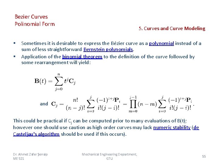
Bezier Curves Polinomial Form § § 5. Curves and Curve Modeling Sometimes it is desirable to express the Bézier curve as a polynomial instead of a sum of less straightforward Bernstein polynomials. Application of the binomial theorem to the definition of the curve followed by some rearrangement will yield: and This could be practical if Cj can be computed prior to many evaluations of B(t); however one should use caution as high order curves may lack numeric stability (de Casteljau's algorithm should be used if this occurs). Dr. Ahmet Zafer Şenalp ME 521 Mechanical Engineering Department, GTU 55

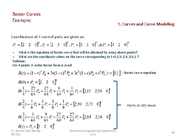
Bezier Curves Example: 5. Curves and Curve Modeling Coordinatess of 4 control poits are given as: What is the equation of Bezier curve that will be obtained by using above points? Ø What are the coordinate values on the curve corresponding to t=0, 1/4, 2/4, 3/4, 1 ? Solution: For 4 points 3. order Bezier form is used: Ø : Bezier curve equation Points on B(t) curve Dr. Ahmet Zafer Şenalp ME 521 Mechanical Engineering Department, GTU 56

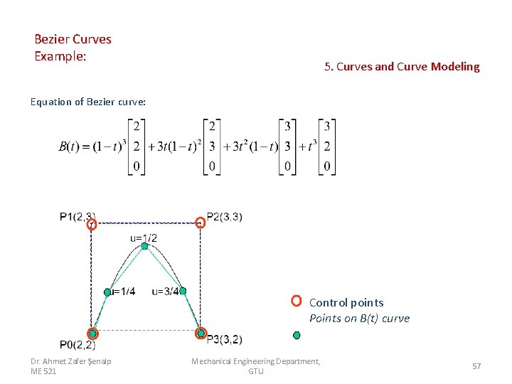
Bezier Curves Example: 5. Curves and Curve Modeling Equation of Bezier curve: Control points Points on B(t) curve Dr. Ahmet Zafer Şenalp ME 521 Mechanical Engineering Department, GTU 57

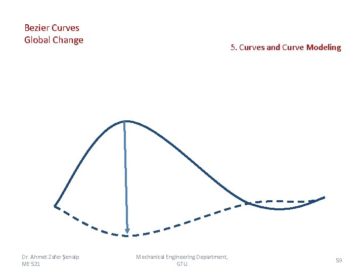
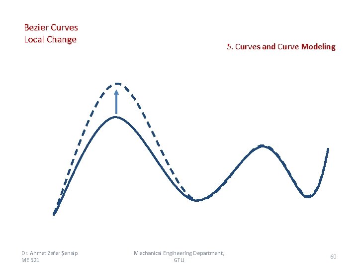
Bezier Curves Disadvantages 5. Curves and Curve Modeling Ï Difficult to interpolate points Ï Cannot locally modify a Bezier curve Dr. Ahmet Zafer Şenalp ME 521 Mechanical Engineering Department, GTU 58

Bezier Curves Global Change Dr. Ahmet Zafer Şenalp ME 521 5. Curves and Curve Modeling Mechanical Engineering Department, GTU 59

Bezier Curves Local Change Dr. Ahmet Zafer Şenalp ME 521 5. Curves and Curve Modeling Mechanical Engineering Department, GTU 60

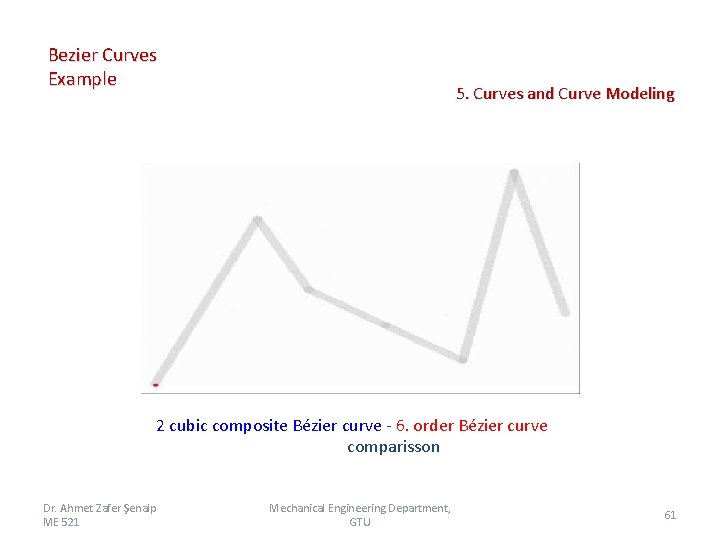
Bezier Curves Example 5. Curves and Curve Modeling 2 cubic composite Bézier curve - 6. order Bézier curve comparisson Dr. Ahmet Zafer Şenalp ME 521 Mechanical Engineering Department, GTU 61

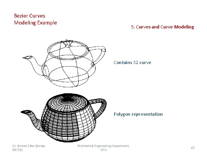
Bezier Curves Modeling Example 5. Curves and Curve Modeling Contains 32 curve Polygon representation Dr. Ahmet Zafer Şenalp ME 521 Mechanical Engineering Department, GTU 62

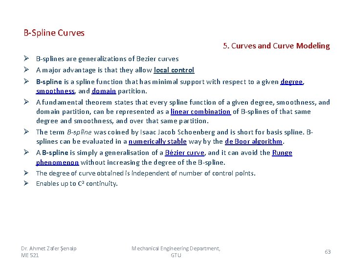
B-Spline Curves 5. Curves and Curve Modeling Ø B-splines are generalizations of Bezier curves Ø A major advantage is that they allow local control Ø B-spline is a spline function that has minimal support with respect to a given degree, smoothness, and domain partition. Ø A fundamental theorem states that every spline function of a given degree, smoothness, and domain partition, can be represented as a linear combination of B-splines of that same degree and smoothness, and over that same partition. Ø The term B-spline was coined by Isaac Jacob Schoenberg and is short for basis spline. Bsplines can be evaluated in a numerically stable way by the de Boor algorithm. Ø A B-spline is simply a generalisation of a Bézier curve, and it can avoid the Runge phenomenon without increasing the degree of the B-spline. Ø The degree of curve obtained is independent of number of control points. Ø Enables up to C 2 continuity. Dr. Ahmet Zafer Şenalp ME 521 Mechanical Engineering Department, GTU 63

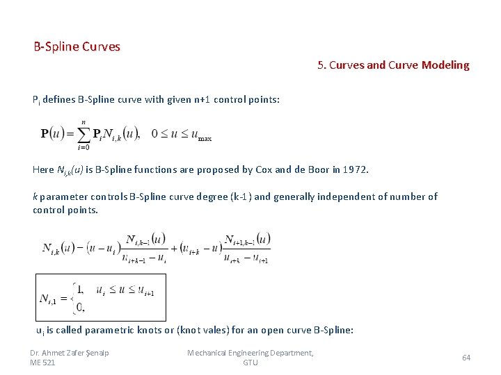
B-Spline Curves 5. Curves and Curve Modeling Pi defines B-Spline curve with given n+1 control points: Here Ni, k(u) is B-Spline functions are proposed by Cox and de Boor in 1972. k parameter controls B-Spline curve degree (k-1) and generally independent of number of control points. aksi durumda ui is called parametric knots or (knot vales) for an open curve B-Spline: Dr. Ahmet Zafer Şenalp ME 521 Mechanical Engineering Department, GTU 64

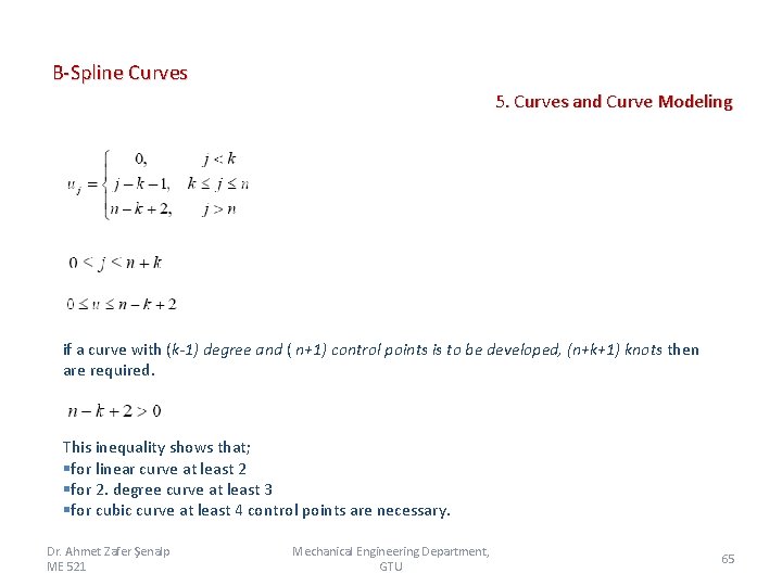
B-Spline Curves 5. Curves and Curve Modeling if a curve with (k-1) degree and ( n+1) control points is to be developed, (n+k+1) knots then are required. This inequality shows that; §for linear curve at least 2 §for 2. degree curve at least 3 §for cubic curve at least 4 control points are necessary. Dr. Ahmet Zafer Şenalp ME 521 Mechanical Engineering Department, GTU 65

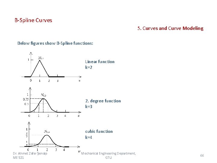
B-Spline Curves 5. Curves and Curve Modeling Below figures show B-Spline functions: Linear function k=2 2. degree function k=3 cubic function k=4 Dr. Ahmet Zafer Şenalp ME 521 Mechanical Engineering Department, GTU 66

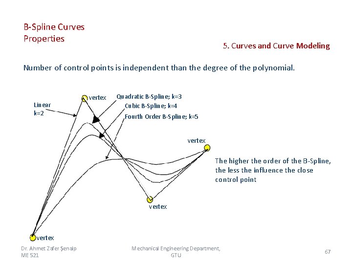
B-Spline Curves Properties 5. Curves and Curve Modeling Number of control points is independent than the degree of the polynomial. Linear k=2 vertex Quadratic B-Spline; k=3 Cubic B-Spline; k=4 Fourth Order B-Spline; k=5 vertex The higher the order of the B-Spline, the less the influence the close control point vertex Dr. Ahmet Zafer Şenalp ME 521 n=3 Mechanical Engineering Department, GTU 67

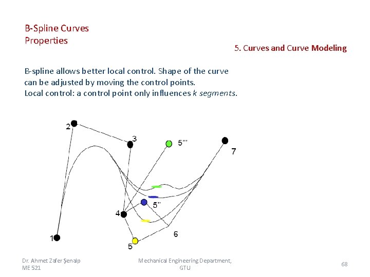
B-Spline Curves Properties 5. Curves and Curve Modeling B-spline allows better local control. Shape of the curve can be adjusted by moving the control points. Local control: a control point only influences k segments. Dr. Ahmet Zafer Şenalp ME 521 Mechanical Engineering Department, GTU 68

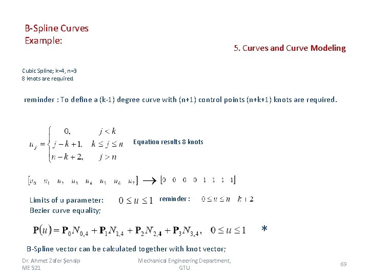
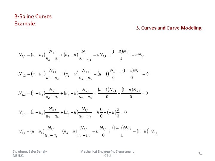
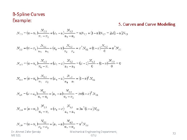
B-Spline Curves Example: 5. Curves and Curve Modeling Cubic Spline; k=4, n=3 8 knots are required. reminder : To define a (k-1) degree curve with (n+1) control points (n+k+1) knots are required. Equation results 8 knots Limits of u parameter: Bezier curve equality; reminder : * B-Spline vector can be calculated together with knot vector; Dr. Ahmet Zafer Şenalp ME 521 Mechanical Engineering Department, GTU 69

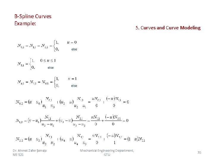
B-Spline Curves Example: 5. Curves and Curve Modeling aksi durumda else Dr. Ahmet Zafer Şenalp ME 521 Mechanical Engineering Department, GTU 70

B-Spline Curves Example: Dr. Ahmet Zafer Şenalp ME 521 5. Curves and Curve Modeling Mechanical Engineering Department, GTU 71

B-Spline Curves Example: Dr. Ahmet Zafer Şenalp ME 521 5. Curves and Curve Modeling Mechanical Engineering Department, GTU 72

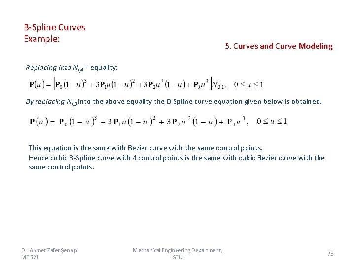
B-Spline Curves Example: 5. Curves and Curve Modeling Replacing into Ni, 4 * equality; By replacing Ni, 3 into the above equality the B-Spline curve equation given below is obtained. This equation is the same with Bezier curve with the same control points. Hence cubic B-Spline curve with 4 control points is the same with cubic Bezier curve with the same control points. Dr. Ahmet Zafer Şenalp ME 521 Mechanical Engineering Department, GTU 73

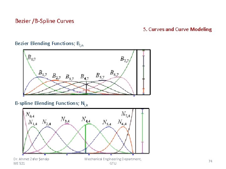
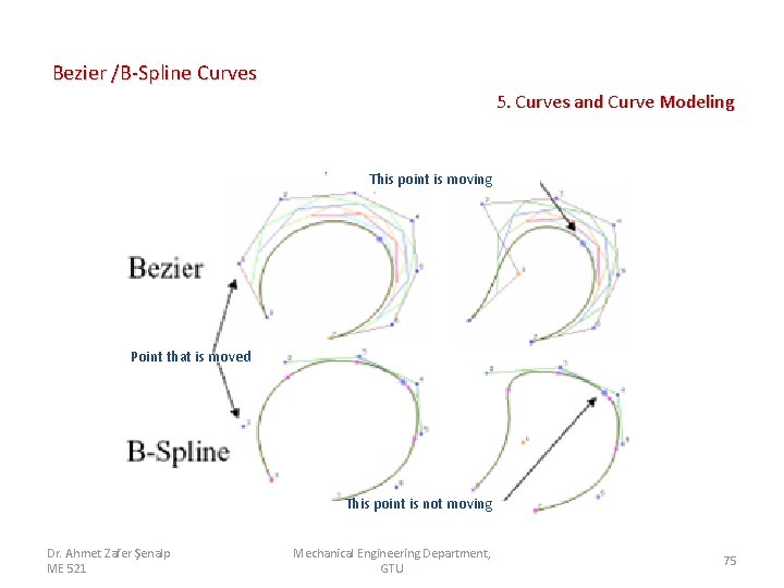
Bezier /B-Spline Curves 5. Curves and Curve Modeling Bezier Blending Functions; Bi, n B-spline Blending Functions; Ni, k Dr. Ahmet Zafer Şenalp ME 521 Mechanical Engineering Department, GTU 74

Bezier /B-Spline Curves 5. Curves and Curve Modeling This point is moving Point that is moved This point is not moving Dr. Ahmet Zafer Şenalp ME 521 Mechanical Engineering Department, GTU 75

Uniform B-Spline Curves 5. Curves and Curve Modeling When B-spline is uniform B-spline functions with n degrees are just shifted copies of each other. Knots are equally spaced along the curve. Dr. Ahmet Zafer Şenalp ME 521 Mechanical Engineering Department, GTU 76

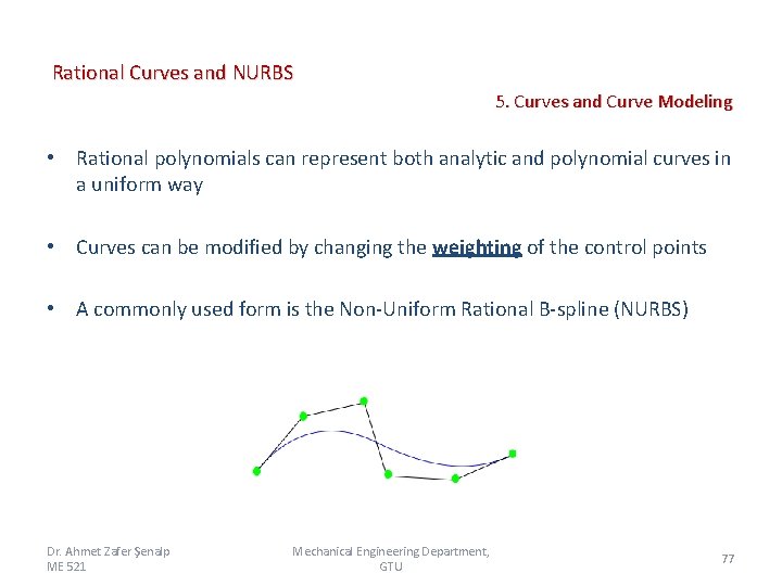
Rational Curves and NURBS 5. Curves and Curve Modeling • Rational polynomials can represent both analytic and polynomial curves in a uniform way • Curves can be modified by changing the weighting of the control points • A commonly used form is the Non-Uniform Rational B-spline (NURBS) Dr. Ahmet Zafer Şenalp ME 521 Mechanical Engineering Department, GTU 77

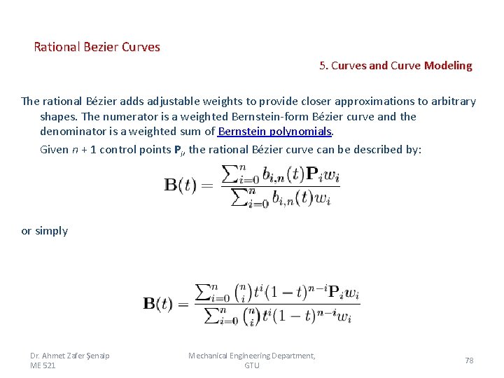
Rational Bezier Curves 5. Curves and Curve Modeling The rational Bézier adds adjustable weights to provide closer approximations to arbitrary shapes. The numerator is a weighted Bernstein-form Bézier curve and the denominator is a weighted sum of Bernstein polynomials. Given n + 1 control points Pi, the rational Bézier curve can be described by: or simply Dr. Ahmet Zafer Şenalp ME 521 Mechanical Engineering Department, GTU 78

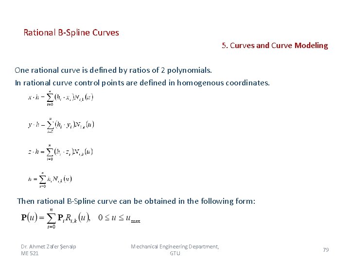
Rational B-Spline Curves 5. Curves and Curve Modeling One rational curve is defined by ratios of 2 polynomials. In rational curve control points are defined in homogenous coordinates. Then rational B-Spline curve can be obtained in the following form: Dr. Ahmet Zafer Şenalp ME 521 Mechanical Engineering Department, GTU 79

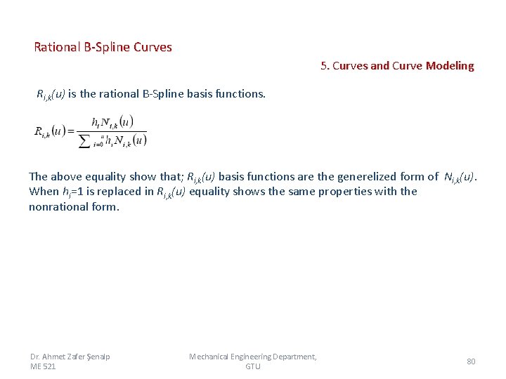
Rational B-Spline Curves 5. Curves and Curve Modeling Ri, k(u) is the rational B-Spline basis functions. The above equality show that; Ri, k(u) basis functions are the generelized form of Ni, k(u). When hi=1 is replaced in Ri, k(u) equality shows the same properties with the nonrational form. Dr. Ahmet Zafer Şenalp ME 521 Mechanical Engineering Department, GTU 80

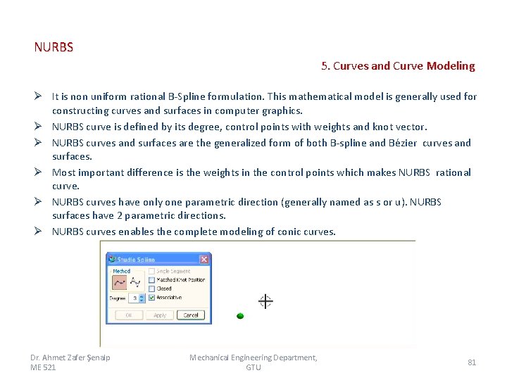
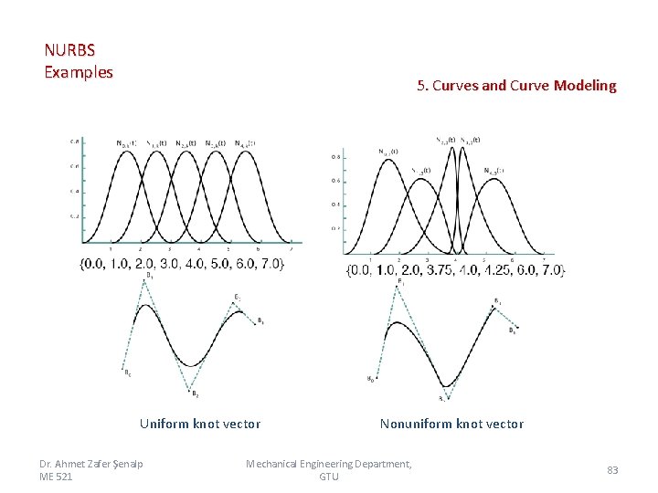
NURBS 5. Curves and Curve Modeling Ø It is non uniform rational B-Spline formulation. This mathematical model is generally used for constructing curves and surfaces in computer graphics. Ø NURBS curve is defined by its degree, control points with weights and knot vector. Ø NURBS curves and surfaces are the generalized form of both B-spline and Bézier curves and surfaces. Ø Most important difference is the weights in the control points which makes NURBS rational curve. Ø NURBS curves have only one parametric direction (generally named as s or u). NURBS surfaces have 2 parametric directions. Ø NURBS curves enables the complete modeling of conic curves. Dr. Ahmet Zafer Şenalp ME 521 Mechanical Engineering Department, GTU 81

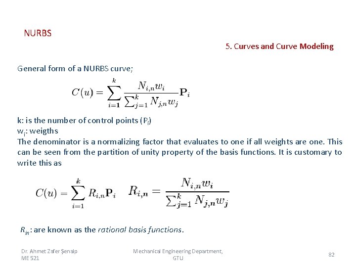
NURBS 5. Curves and Curve Modeling General form of a NURBS curve; k: is the number of control points (Pi) wi: weigths The denominator is a normalizing factor that evaluates to one if all weights are one. This can be seen from the partition of unity property of the basis functions. It is customary to write this as Rin: are known as the rational basis functions. Dr. Ahmet Zafer Şenalp ME 521 Mechanical Engineering Department, GTU 82

NURBS Examples 5. Curves and Curve Modeling Uniform knot vector Dr. Ahmet Zafer Şenalp ME 521 Nonuniform knot vector Mechanical Engineering Department, GTU 83

NURBS Development of NURBS 5. Curves and Curve Modeling Ø Ø Boeing: Tiger System in 1979 SDRC: Geomod in 1993 University of Utah: Alpha-1 in 1981 Industry Standard: IGES, PHIGS, PDES, Pro/E, etc. Dr. Ahmet Zafer Şenalp ME 521 Mechanical Engineering Department, GTU 84

NURBS Advantages 5. Curves and Curve Modeling ü Serve as a genuine generalizations of non-rational B-spline forms as well as rational and non-rational Bezier curves and surfaces ü Offer a common mathematical form for representing both standard analytic shapes (conics, quadratics, surface of revolution, etc) and free-from curves and surfaces precisely. B-splines can only approximate conic curves. ü By evaluating a NURBS curve at various values of the parameter, the curve can be represented in cartesian two- or three-dimensional space. Likewise, by evaluating a NURBS surface at various values of the two parameters, the surface can be represented in cartesian space. ü Provide the flexibility to design a large variety of shapes by using control points and weights. increasing the weights has the effect of drawing a curve toward the control point. Dr. Ahmet Zafer Şenalp ME 521 Mechanical Engineering Department, GTU 85

NURBS Advantages 5. Curves and Curve Modeling ü Have a powerful tool kit (knot insertion/refinement/removal, degree elevation, splitting, etc. ) ü They are invariant under affine as well as perspective transformations: operations like rotations and translations can be applied to NURBS curves and surfaces by applying them to their control points. ü Reasonably fast and computationally stable. They reduce the memory consumption when storing shapes (compared to simpler methods). ü They can be evaluated reasonably quickly by numerically stable and accurate algorithms. ü Clear geometric interpretations Dr. Ahmet Zafer Şenalp ME 521 Mechanical Engineering Department, GTU 86