18 Curves and Surfaces II Based on EA

计算机图形学讲义－18 Curves and Surfaces (II) 姜明 北京大学数学科学学院 Based on [EA], Chapter 11. 更新时间 2020/10/30 5: 13: 33

计算机图形学讲义－18 Outline • • Hermite Curves and Surfaces Bezier Curves and Surfaces Cubic B-Splines General B-Splines

计算机图形学讲义－18 Hermite Curves and Surfaces • Given the control points p 0 and p 3. • Request interpolating conditions at u = 0 and u = 1 for the given control-point data. • Two other conditions: we assume that the derivatives at u = 0 and u = 1 are given.

计算机图形学讲义－18 In most interactive applications, however, the user enters point data rather than derivative data, unless analytical formulations of the data are available. MH is the Hermite geometry matrix.

计算机图形学讲义－18 Blending Functions matlab program

计算机图形学讲义－18 Geometric and Parametric Continuity • Various continuity conditions by matching the polynomials and their derivatives at u = 1 for p(u) and corresponding values for q(u) at u = 0. C 0=G 0 C 1 G 1

计算机图形学讲义－18 G 1 Is Useful • Here the p and q have the same tangents at the ends of the segment but different derivatives. - they generate different Hermite curves. • This technique is used in drawing applications, - the user can interactively change the magnitude, leaving the tangent Angel: Interactive Computer Graphics 5 E © Addison-Wesley 2009 direction unchanged 7

计算机图形学讲义－18 G 1 Might be Worse than C 1 G 1 • However, in other applications, such as animation, where a sequence of curve segments describes the path of an object. • G 1 continuity may be insufficient. • we might see changes in velocity as objects move along paths described with only G 1 continuity.

计算机图形学讲义－18 Bezier Curves and Surfaces • Given 4 control points p 0, p 1, p 2 and p 3. • Request interpolating conditions at end points. • Bezier suggested to use p 1 and p 2 to approximate the tangents at u = 0 and u = 1.

计算机图形学讲义－18 For a set of control points, we can have C 0 continuity at joint points with Bezier splines, but we have given up the C 1 continuity. MB is the Bezier geometry matrix.

计算机图形学讲义－18 Blending Functions matlab program

计算机图形学讲义－18 Bernstein polynomials p(u) must lie in the convex hull of the four control points. http: //en. wikipedia. org/wiki/Bernstein_polynomial

计算机图形学讲义－18 Bezier Surface Patch lies in the convex hull of the control points. It is a measure of the tendency of the patch to divert from being flat, or to twist, at the corner.

计算机图形学讲义－18 Limitations of Bezier Curves/Surfaces • In practice, the cubic Bezier curves and surface patches are widely used. • One fundamental limitation – at the join points (or patch edges, for surfaces), we have only C 0 continuity. • It might seem – the limit of what we can do with cubic parametric polynomials, – high-degree polynomials or shorten the interval and use more polynomial segments, for more flexibility. • Another approach – we can use the same control-point data but not require the polynomial to interpolate any of these points. – If we can come close to the control points and get more smoothness at the join points.

计算机图形学讲义－18 Cubic B-Splines • • • The Cubic B-Spline Curve B-Splines and Basis. matlab program Spline Surfaces

计算机图形学讲义－18 The Cubic B-Spline Curve • Consider 4 control points from a sequence of control points. • Instead of interpolating at end points, only generate a curve inside the convex hull as u goes from 0 to 1.

计算机图形学讲义－18 Adding Points • One new control point will generate a new patch of spline. • {pi-3, pi-2, pi-1, pi} generates the first curve q(u). . • {pi-2, pi-1, pi+1} generates the second curve p(u).

计算机图形学讲义－18 • We match conditions at q(1) and p(0). • q(1) = p(0), requires continuity at the joint point, without requiring interpolation of any data. • There are many sets of conditions; each set can define a different spline. • We derive the most popular spline, by assuming that the spline treat symmetrically to points at each side of the joint point.

计算机图形学讲义－18 - Any evaluation of conditions on q(1) cannot use pi-3, because this control point does not appear in the equation for p(u). - Likewise, we cannot use pi+1 in any condition on p(0).

计算机图形学讲义－18 MS is the B-spline geometry matrix.

计算机图形学讲义－18 Blending Functions matlab program

计算机图形学讲义－18 Contribution of Control Points • Each control point contributes to the spline in four adjacent intervals of the parameter u. for the whole curve. • This property guarantees the locality of the spline. • • For the control point pi. Contribution to p(u) is weighted by b 2(u), in [0, 1]. Contribution to q(u) with weigh b 3(u+1) in [-1, 0]. The shift of u by 1 from [-1, 0] to [0, 1] is to compute the contribution to the whole curve with one parameter u.

计算机图形学讲义－18 Contributions of pi to • p(u) weighted by b 2(u), in [0, 1]. • q(u) weighted by b 3(u+1) in [-1, 0]. - - The shift of u by 1 from [-1, 0] to [0, 1] is necessary to formulate to the whole curve with one parameter u.

计算机图形学讲义－18 Control Point and Basis Function • For the control point pi. - • Its contribution to the whole curve is weighted by bi(u), i = 0, 1, 2, 3, depending on its relative position in the curve segment. • If we shift the parameter u by 1 to each left interval consequently, the - contribution of pi to the total curve can be written as Bi(u) pi.

计算机图形学讲义－18 - the function Bi(u) and the contribution from the individual basis and control point. - End points to be discussed later.

计算机图形学讲义－18 Comments on the Cubic B-splines • In fact, it is C 2. • It is for this reason that spline curves are so important. • From a physical point of view, metal will bend such that the second derivative is continuous. • From a visual perspective, a curve made of cubic segments with C 2 continuity will be seen as smooth, even at the join points.

计算机图形学讲义－18 Properties • p(u) must lie in the convex hull of the four control points. • The curve from a set of control points has C 1 continuity. • The curve only approximates well the middle two points as u goes from 0 to 1. • we are doing three times the work that we would do for Bezier or interpolating cubics.

计算机图形学讲义－18 Cubic B-spline Surface Patch defined over only 1/9 of region.

计算机图形学讲义－18 General B-Splines • • - Recursively Defined B-splines Uniform Splines Nonuniform B-Splines NURBS A History of Curves and Surfaces in CAGD by Gerald Farin

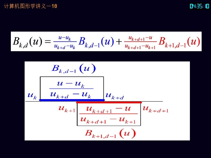
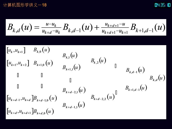
计算机图形学讲义－18 Recursively Defined B-splines • The blending functions for B-splines form a basis set. – The “B” in B-spline is for “basis” • Given knot sequence • Cox-de Boor recursion Define */0=0 in this formula.

计算机图形学讲义－18 Example • If the degree is zero (i. e. , d = 0), basis functions are step functions. Copy-edited from http: //www. cs. mtu. edu/~shene/COURSES/cs 3621/NOTES/spline/B-spline/bspline-basis. html

计算机图形学讲义－18 Examples - Further Examples http: //www. cs. mtu. edu/~shene/COURSES/cs 3621/NOTES/spline/B-spline/bspline-ex-1. html

计算机图形学讲义－18 Properties of General B-Splines Copy-edited from http: //www. cs. mtu. edu/~shene/COURSES/cs 3621/NOTES/spline/B-spline/bspline-basis. html http: //www. cs. mtu. edu/~shene/COURSES/cs 3621/NOTES/spline/B-spline/bspline-property. html

计算机图形学讲义－18 General B-spline curves • Given n+1 points • Polynomials of d-th degree in n intervals [uk, uk+1], k = 0, …, m, with n+1 knots. – Each control point needs a basis function and the number of basis functions satisfies n + 1 = m - d. • The name B-splines comes from the term basis splines • The set of functions {Bi, d(u)} forms a basis for the given knot sequence and degree.

计算机图形学讲义－18 Properties of B-spline curves • A B-spline curve is a piecewise curve with each component a curve of degree d. • A B-spline curve is contained in the convex hull of its control points. • p(u) is Cd-k continuous at a knot of multiplicity k. • Geometric smoothness of B-spline curves can be further studied by its derivatives and additional geometry conditions on control points, such as clamped B-spline curves. http: //www. cs. mtu. edu/~shene/COURSES/cs 3621/NOTES/spline/B-spline/bspline-derv. html

计算机图形学讲义－18 Control Parameters • The degree of B-spline basis functions is only an input. • To change the shape of a B-spline curve, one can modify one or more of these control parameters: – the positions of control points, – the number and positions of knots – the degree of the curve. Copy-edited from http: //www. cs. mtu. edu/~shene/COURSES/cs 3621/NOTES/spline/B-spline/bspline-curve. html

计算机图形学讲义－18 Uniform Splines

计算机图形学讲义－18 Open Splines • If the control points do not have any particular structure, the generated curve will not touch the first and last legs of the control polyline. • This type of B-spline curves is called open B-spline curves. n = 9, d = 3, m+1 = 14. Copy-edited from http: //www. cs. mtu. edu/~shene/COURSES/cs 3621/NOTES/spline/B-spline/bspline-curve. html

计算机图形学讲义－18 Clamped B-spline curves • To get a curve that is tangent to the first and the last legs at the first and last control points, as a Bézier curve does. • The first knot and the last knot must be of multiplicity d+1. • This will generate the so-called clamped B-spline curves. • By repeating some knots and control points, the generated curve can be a closed one. • Clamp: 夹钳 first d+1 = 4 and last 4 knots must be identical. The remaining 14 - (4 + 4) = 6 knots can be anywhere. { 0, 0, 0. 14, 0. 28, 0. 42, 0. 57, 0. 71, 0. 85, 1, 1 }. Copy-edited from http: //www. cs. mtu. edu/~shene/COURSES/cs 3621/NOTES/spline/B-spline/bspline-curve. html http: //www. cs. mtu. edu/~shene/COURSES/cs 3621/NOTES/spline/B-spline/bspline-derv. html

计算机图形学讲义－18 Nonuniform B-Splines • Repeated knots have the effect of pulling the spline closer to the control point associated with the knot. • If a knot at the end has multiplicity d + 1, the B-spline of degree d must interpolate the point. • The knot sequence {0, 0, 1, 2 , . . . , n - 1, n, n} is often used for cubic B-splines. • For the sequence {0, 0, 1, 1, 1, 1} the cubic B-spline becomes the cubic Bezier. – Proof.

计算机图形学讲义－18 NURBS • Nonuniform rational Bspline. • It has the convex-hull and continuity properties. • It can be handled correctly in perspective views. • wi weights the impact of the point pi.